0. Executive Summary & Key Findings
There is nothing mystical about Bitcoin's price cycles. They are the visible surface of capital flowing into a fixed-supply asset and of long-term holders deciding when, and how much, to sell. The Blocklens-TOP model formalizes both halves of that statement into a single, closed system — and reproduces the full Bitcoin price cycle, bottom and top alike, from one set of parameters grounded in the historical on-chain behavior of market participants.
Historically, on-chain analysis has been good at identifying the cycle bottom, but until now there has been no precise model for locating a potential cycle top from holder behavior. The Blocklens-TOP model is built to close that gap, and it lets you answer two interlocking questions:
- What top price can bitcoin be expected to reach if \$X billion of capital enters the asset?
- What capital inflow must the coming cycle deliver for bitcoin's price to exceed \$Y thousand?
The model in a nutshell
The Blocklens-TOP model is a two-phase description of the complete cycle (descent and ascent), and each phase is driven mainly by the behavior of the same cohort: long-term holders.
- Tops form endogenously, mainly through distribution feedback from Long-Term Holders (LTH). As price climbs, long-term holders sit on larger unrealized gains, measured by their MVRV (market value to realized value — price divided by the LTH cost basis). Higher MVRV makes them sell faster. That extra selling raises the market's daily "spend volume" of bitcoin, which mathematically damps how fast new capital can push price higher. Price growth decelerates and a top forms — not because of an external shock, but because the cohort's own profit-taking closes a negative feedback loop. We capture this with a gentle power law, \(c_{LTH}=0.093\cdot \text{MVRV}_{LTH}^{\,0.27}\) (binned R²≈0.857), where \(c_{LTH}\) is the fraction of LTH supply spent per day.
- Bottoms form at the LTH cost-basis floor. A cycle ends when long-term holders are deep enough underwater that the selling exhausts itself. The bottom price is the LTH realized price multiplied by a floor multiple (marking the depth of LTH losses at which buying to average down those positions starts to dominate), \(p_{bottom} = \text{MVRV}_{\text{LTH}}^{\text{floor}}\times RP_{LTH}\). Crucially, realized cap is sticky through a bear market — it barely falls. A crash is a market-cap collapse, not a realized-cap one, which is exactly why a cost-basis floor anchors the bottom.
Both phases plug into one exact mathematical identity. By definition, the daily change in realized cap equals realized profit/loss plus issuance; solving that identity for price yields the model's anchor equation:
$$ p_t = \text{inertia}(t) + \frac{\Delta \mathrm{RCap}(t)}{Q(t)} \tag{1}$$Here \(\Delta\text{RCap}(t)\) is the day's change in realized cap (a proxy for capital inflow/outflow), \(Q(t)\) is the market's daily spend volume in BTC, and "inertia" is the spend-weighted cost basis the market is selling from.
Walk-forward: out-of-sample validation
The real test of any cycle model is whether it can forecast a top it has never seen. We refit every parameter using only data from before each predicted cycle, with no future leakage, and test the model out-of-sample. From the future the model receives the actual total capital inflow for the cycle (\(\Delta RCap\) from bottom to top) and its calendar (the bottom and top dates); the inflow is itself partially endogenous to price — realized profit scales with the price path — so the test should be read as a transfer-function test of “inflow → price”, not as a full forecast of the future. This lets us compare \( p_{\text{model}}^{\text{TOP}}(\Delta RCap_{\text{actual}}) \) with \( p_{\text{actual}}^{\text{TOP}} \):
| Predicted top | Out-of-sample error | Note |
|---|---|---|
| 2017 | −26% | Only the extreme 2013 cycle as prior |
| 2021 | +10% | The regime-shift cycle (deployment profile collapsed mid-cycle) |
| 2025 | −1% | Trained only on data through 2022 — the headline result |
The 2025 prediction is the one that matters: a modern cycle, forecast from a clean prior cycle, landed within 1%. The misses on the earlier cycles are explainable — 2017 had only the anomalous early market to learn from, and 2021 turned out to be a genuine structural break in the pattern of capital inflow (the deployment exponent \(K\) fell from ~7 to ~2.7 mid-cycle, unknowable from history).
Forward forecast
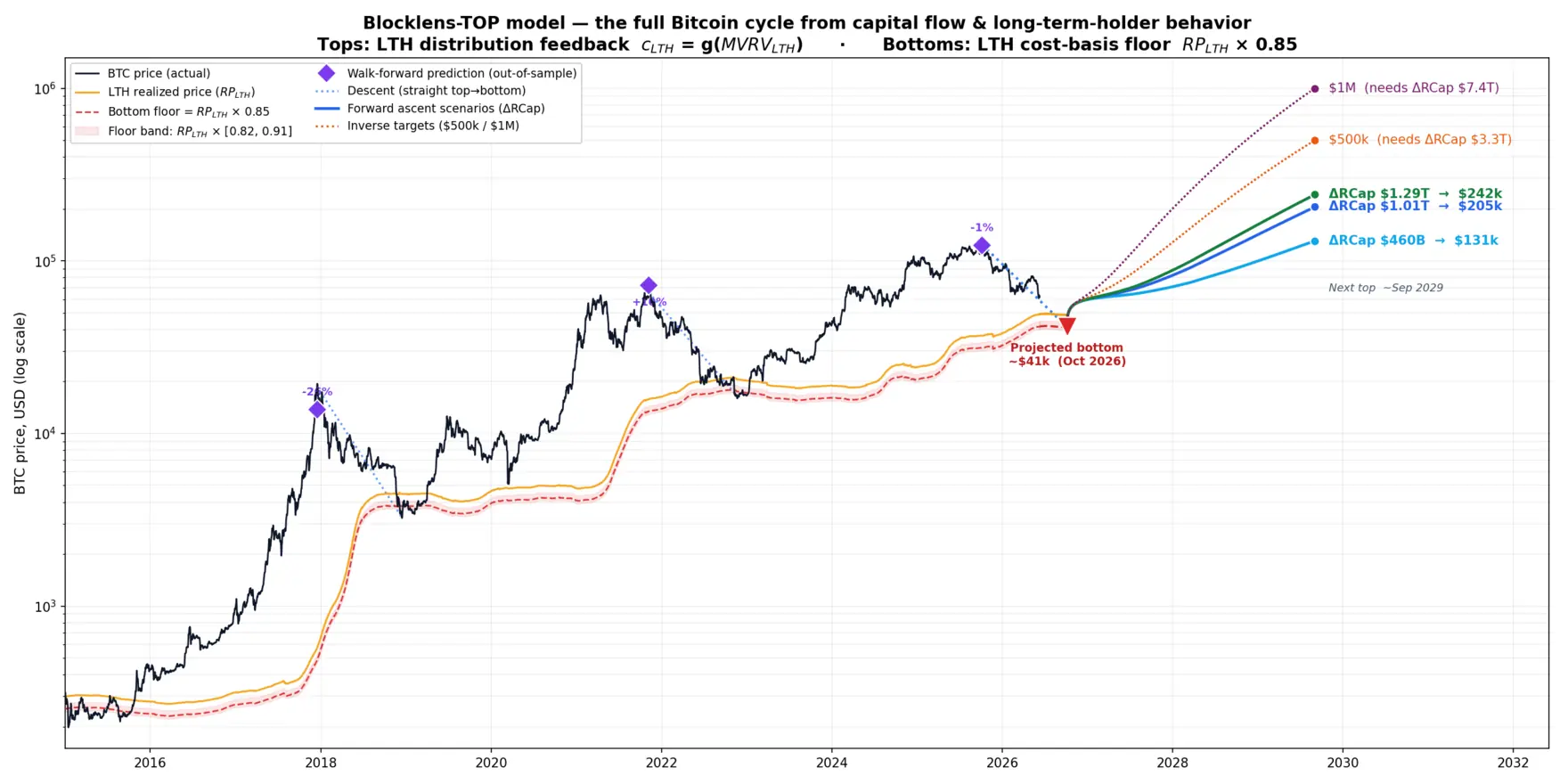
Bitcoin's most recent top printed at \$124,414 on October 6, 2025. The descent into mid-2026 has carried the price to \$61.7k (data cutoff: June 10, 2026). From here the model projects the cycle bottom (no capital-inflow assumptions required) and the subsequent cycle top as a function of the capital inflows assumed for the coming ascent:
- Bottom: ≈ \$41k (the floor band gives \$39–44k; with the \(RP_{LTH}\) annual forecast error — roughly \$36–47k) expected in October 2026 — exactly one year after the top, consistent with the remarkably stable ~365-day modern descent (363 and 366 days in the two completed cases). The LTH cost basis climbs to \( RP_{LTH} \) ≈ \$48.6k by then.
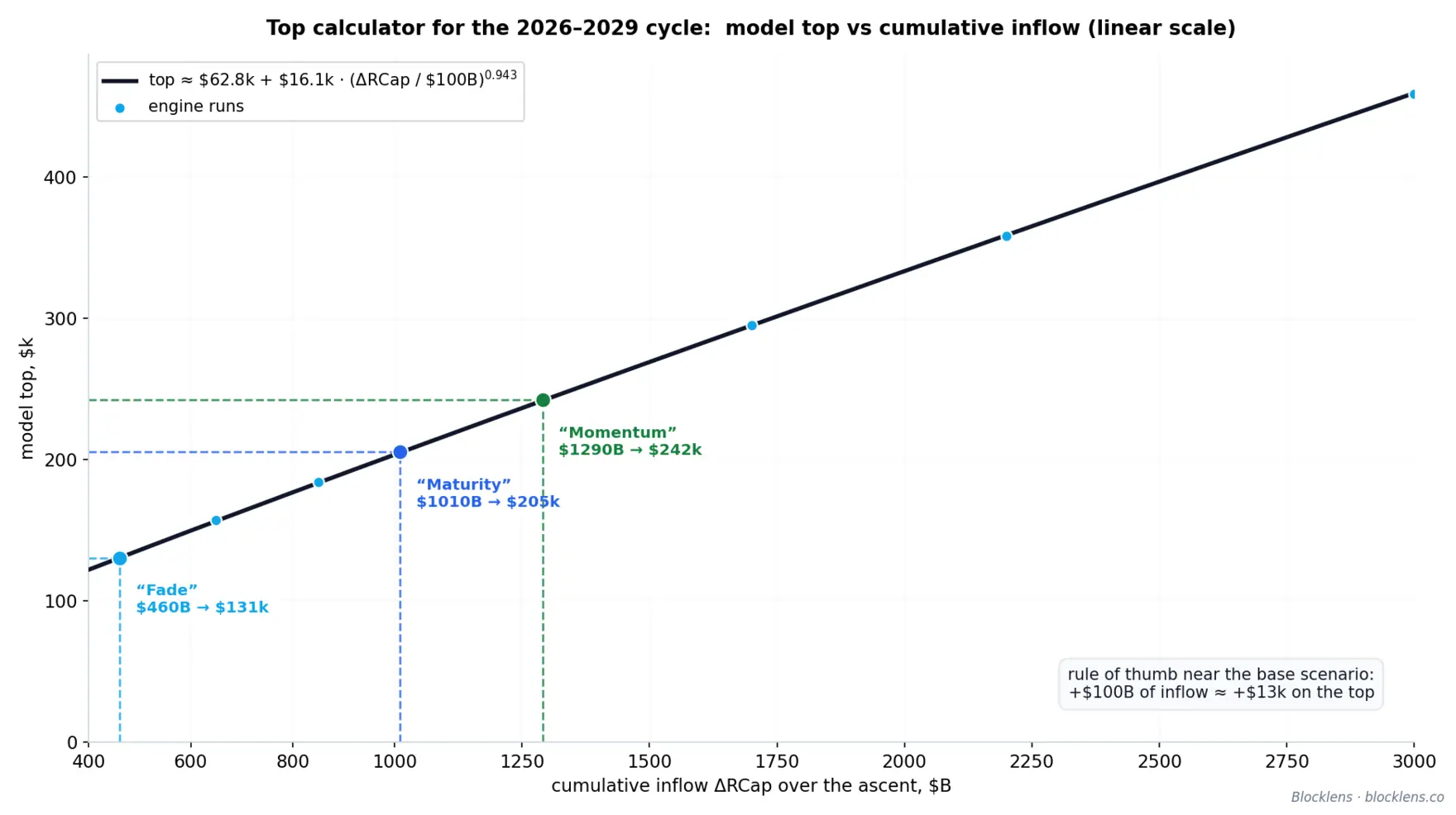
- Next top (conditional on capital inflows): the scenarios are anchored to the actual inflows of past cycles (\$69B → \$364B → \$685B). The conservative “Fade” (\$460B, the inflow multiplier's decay repeats) implies ~\$131k — only ~5% above the 2025 top; the central “Maturity” (\$1.01T, the inflow increment repeats) ~\$205k; the optimistic “Momentum” (\$1.29T, the prior cycle's multiplier repeats) ~\$242k. You can also compute the capital inflow required for bitcoin to reach a given level in the coming cycle: \$500k/BTC would take ≈\$3.3T of deployment into realized cap, and \$1M/BTC ≈\$7.4T.
These top figures are explicitly conditional: the point of the model is to pin down the interdependence of price and capital inflow — it is not an autonomous oracle. It tells you what price the market should reach at the top for a given wave of capital inflow (and, conversely, what inflow it takes to hit a given top price in the coming cycle), but it does not pretend to know how much capital market participants will commit to bitcoin; that is a question for our future research.
Main contributions
- An endogenous theory of cycle tops. Tops are the fixed point of an LTH distribution feedback loop, \(c_{LTH}=g(\text{MVRV})\), rather than the product of arbitrary indicators or of any external trigger beyond capital inflow itself.
- A cost-basis theory of cycle bottoms. The bottom is set by a 15% discount to the LTH cost basis. The cost basis itself can be approximated well up to a year ahead via LTH realized-cap accounting (the RCLTH ledger).
- The −1% out-of-sample 2025 top. A genuine out-of-sample walk-forward test of a modern cycle top, trained only on prior data — compelling evidence that the mechanism is real.
- A sensitivity law for the daily spend volume \(Q\). Each driver's impact equals its coefficient of variation times its weight in \(Q\); this cleanly separates what sets \(Q\)'s level (short-term-holder spending) from what forms the top (long-term-holder spending) — telling you where to model in detail and where you can afford to simplify.
- Cohort effective realized cost bases and their kernels as standalone metrics. The STH effective realized cost basis (\(p_{SOPR}^{STH}\)) is well approximated by a short, front-loaded average of recent price (R²≈0.9995); the LTH effective realized cost basis (\(p_{SOPR}^{LTH}\)) is approximated by a bell-kernel of price at long lag (R²≈0.92 raw, ≈0.98 smoothed) — the bell arising naturally as the derivative of the logistic aging weight.
- A quantitative account of market maturation. Top \( MVRV_{LTH} \) has compressed across cycles (34 → 33 → 4.1 → 3.4) while the bottom floor has risen (0.66 → 0.82) and capital deployment has grown more even (the deployment-curve steepness \(K\) declines: ~7 → ~2.75) — drawdowns shrink as absolute price levels climb. The model can predict the expected top \( MVRV_{LTH} \), since that parameter is an endogenous variable (under “Fade” at \$460B, \( MVRV_{LTH} \) ~ 2.49; under “Maturity” at \$1.01T, ~3.28; under “Momentum” at \$1.29T, ~3.57).
The sections that follow build the model from the bottom up, starting from the mathematical foundations: the cohort split and cost-basis kernels, the equation linking the price law to capital inflow, the LTH distribution feedback that forms tops, the cost-basis multiple that forms bottoms, and the full validation — both on the training history and in out-of-sample walk-forward mode.
1. Prior Work: Reading Tops and Bottoms On-Chain
On-chain analysis began with a simple, radical premise: a public blockchain records every coin's last movement, so the cost basis of the entire money supply is, in principle, knowable. From that premise grew an entire family of valuation metrics. Each one has earned its place. But almost all of them share a quiet limitation: they describe the market's state without explaining how that state came to be. This section walks through the lineage that the Blocklens-TOP model inherits, and then names the gap it was built to close.
1.1 Realized Cap and Realized Price
The foundational move was to stop valuing coins at today's price and start valuing them at the price at which each coin last moved. Coin Metrics formalized this as Realized Capitalization (Realized Cap, RCap): the sum over all unspent outputs of each coin's quantity times the price on the day that output was created. Where market capitalization (price times circulating supply) answers "what is the supply worth now?", Realized Cap answers "what did the supply cost its holders?" — an aggregate of the network's paid-in capital rather than its mark-to-market valuation.
Dividing Realized Cap by circulating supply yields Realized Price (RP), the network-wide average cost basis per coin. Realized Price behaves like a center of gravity for the market: a soft floor in bear markets, a level the spot price repeatedly tests and bounces off. Both metrics turn the blockchain into an accounting record of investor cost, and many of the metrics that follow are, in some sense, a ratio or a partition of these two.
1.2 MVRV and the MVRV Z-Score
If Realized Cap is what the supply cost and market cap is what it is worth, their ratio measures aggregate unrealized profit. This is the MVRV ratio (Market-Value-to-Realized-Value):
$$\text{MVRV} = \frac{\text{Market Cap}}{\text{Realized Cap}} = \frac{\text{price}}{\text{Realized Price}}.\tag{2}$$MVRV above 1 means the average coin sits in profit; below 1, in loss. Historically, extreme highs have flagged euphoric tops and readings under 1 have marked capitulation bottoms. To sharpen the signal, Awe and Wonder introduced the MVRV Z-Score, which standardizes the gap between market value and realized value by its own historical standard deviation \(\sigma\):
$$\text{MVRV Z} = \frac{\text{Market Cap} - \text{Realized Cap}}{\sigma(\text{Market Cap})}.\tag{3}$$The Z-score has a deserved reputation for calling cycle extremes. Yet it remains a normalized oscillator: it tells you the market is statistically overheated relative to its own past, not what inflow of capital produced the overheating, nor when it must fade. It reads the temperature; it does not model how the fire spreads.
1.3 SOPR: realized profit at the moment of spending
The metrics above value coins that sit still. Renato Shirakashi's Spent Output Profit Ratio (SOPR) values coins the moment they move. For every output spent on a given day, SOPR compares the price at which it was sold to the price at which it was created:
$$\text{SOPR} = \frac{\text{price at spend}}{\text{price at creation}} \;=\; \frac{\text{realized value}}{\text{value paid}}.\tag{4}$$A SOPR above 1 means coins are, on average, being spent in profit; below 1, at a loss; and the line at 1 — the level where sellers merely break even — acts as recurring support in bull markets and resistance in bear markets, as participants rush to exit at break-even. SOPR is important to our work for a specific reason: it is built from the cost basis of spent coins (we introduce the notion of an effective realized cost basis, as distinct from the ordinary cost basis of held coins) — the very birth price of the unspent transaction outputs that, properly cohort-weighted, drive the change in Realized Cap. We adopt this effective realized cost basis of spent coins (denoted \(p_{\text{SOPR}}\)) as a first-class quantity rather than substituting the cost basis of the remaining holdings for it — a distinction we make precise in later sections.
1.4 Holder cohorts and the ~155-day boundary
A further refinement partitions the supply by coin age — the number of days since a coin last moved — into Short-Term Holders (STH) and Long-Term Holders (LTH). The empirical boundary sits near 155 days (Schultze-Kraft, March 2020): beyond roughly five months, the probability that a coin moves again drops sharply, so older coins behave like conviction holdings and younger coins like active, reactive capital. Splitting Realized Price, SOPR, and MVRV along this line produces cohort-specific cost bases and profit ratios — MVRVLTH, STH-SOPR, and so on — that isolate the behavior of the two populations whose interaction drives the cycle.
The 155-day threshold was originally applied as a hard cutoff; a smoothing methodology was proposed later (Heeg & Schultze-Kraft, November 2020). Throughout this report we use a smooth logistic weight on coin age \(a\): \(W_{\text{LTH}}(a) = 1/\left(1 + e^{-0.1(a-155)}\right)\), clamped to 0 below 100 days and 1 above 210 days, with STH weight \(1 - W_{\text{LTH}}\). Smoothing the boundary is a tacit convention among on-chain analysts; it preserves the familiar ~155-day soft boundary (by BTC value) while replacing a discontinuous step with a differentiable transition — and, as later sections show, it is precisely this property that lets us approximate the cohorts' realized cost bases.
1.5 HODL waves and coin-age bands
Rather than collapse age into two cohorts, the HODL waves visualization (Unchained Capital) plots the full distribution of supply across age bands — coins last moved within a day, a week, a month, on up to multiple years — as a stacked, multicolored time series. The picture is vivid: thick young bands swell as speculative coins change hands near a top, then thin out as those coins mature and the old-coin bands thicken through a bear market. HODL waves make the migration of supply between cohorts legible at a glance, and they motivate a key object in our model — the daily churn of aging coins across the STH/LTH boundary. But as a chart, they remain descriptive: a beautiful map of where coins are, not a law for where they go.
1.6 The Time-is-Money spend-hazard view
A more dynamic strand, associated with the Time-is-Money framing (first introduced by Glassnode in 2024), treats bitcoin spending as a hazard process: it asks, for a coin of a given age, what the probability is that it moves today. This spend-hazard view, kin to the coin-days-destroyed tradition, correctly recognizes that older coins are less likely to move and that age-conditioned spending propensities carry information about holder conviction. It points in the right direction — toward behavior, toward flow, toward coins as a population with age-dependent dynamics. In this report we propose a way to connect those spend propensities, through Realized Cap, to the price itself.
1.7 The gap: descriptive oscillators versus a generative engine
Step back and a pattern is clear. Realized Cap and Realized Price are accounting aggregates. MVRV, the Z-score, and SOPR are ratios built on them — oscillators that swing high near tops and low near bottoms. Cohort splits, HODL waves, and spend-hazard curves enrich the description with age structure and behavior. Every one of these tools is a reading of the market's state.
None of them is a mechanism. Each answers "where are we relative to history?" by way of a threshold, a band, or a standardized deviation — and a threshold is a description dressed as a forecast. There are three recurring limitations:
- They are diagnostic, not generative. An oscillator can be stretched, but it does not say what inflow of capital stretched it, nor does it reproduce the price path that the inflow implies.
- Tops and bottoms are read off heuristically. "MVRV is high," "SOPR reset to 1," "the young-cohort bands are thick" — these are pattern-matched against prior cycles. The turning point is recognized, not produced by the model's own internal dynamics.
- They are calibrated, not closed. No conservation identity ties the metrics together, so each is tuned to history independently, and there is no guarantee the pieces are mutually consistent.
The Blocklens-TOP model is built to close exactly this gap. It begins from an exact mathematical identity — the daily change in Realized Cap equals cohort-weighted realized profit/loss plus issuance — and inverts it to express price as a function of capital inflow. Within that engine, the long-term-holder cohort distributes coins faster as their unrealized return rises (a power-law response of the LTH spend rate to MVRVLTH), which raises the system's overall daily spend volume and damps further price growth. A cycle top is therefore not a threshold that gets crossed; it is an equilibrium that the model's own negative feedback produces endogenously. The same mechanism in mirror image shapes the cycle bottom, which forms where long-term holders' unrealized loss reaches levels at which averaging-down sentiment takes over the cohort (a falling spend rate). The metrics surveyed above are not discarded — Realized Cap, Realized Price, SOPR, the cohort split, and MVRVLTH all reappear as load-bearing components. The difference is that here they are wired together by an identity into a single generative model that reproduces the price path, rather than standing apart as separate gauges to be eyeballed at the extremes.
2. A Two-Cohort Model for the Cycle Top
The Bitcoin cycle is, at heart, an exercise in accounting: how much fresh capital has come onto the chain, who is spending coins, and at what price those coins last moved. The Blocklens-TOP model makes this picture exact. We split the supply into two behavioral cohorts, write down the one identity that the Realized Cap (RCap) must obey by definition, and then invert it to recover price as the ratio of capital inflow to daily spend volume. Everything that follows in this report — the coin-spending feedback that forms the top and the cost-basis floor that forms the bottom — hangs on the three design choices laid out here.
Splitting the supply: Short-Term and Long-Term Holders
Every coin carries an age \(a\) — the number of days since it last moved on-chain. Coins that have sat untouched for a long time behave differently from coins that changed hands last week: the old coins belong to conviction holders who sell rarely and reluctantly, the young coins to traders, speculators, and the churn of exchange flow. We call the first group Long-Term Holders (LTH) and the second Short-Term Holders (STH), and we apportion each coin between the two cohorts not with a hard cutoff but with a smooth logistic weight (a sigmoid) on age:
$$ W_{\mathrm{LTH}}(a) = \frac{1}{1 + e^{-0.1\,(a - 155)}} \tag{5}$$Here \(W_{\mathrm{LTH}}(a)\) is the fraction of a coin of age \(a\) counted as long-term-held; the short-term weight is simply \(W_{\mathrm{STH}}(a) = 1 - W_{\mathrm{LTH}}(a)\). The curve is clamped to \(0\) below 100 days and to \(1\) above 210 days, so very young coins are purely short-term and well-aged coins are purely long-term, with a graded transition between the extremes. The crossover sits near \(a \approx 155\) days — the soft STH/LTH boundary in terms of BTC value (a bitcoin aged 155 days counts exactly 50% toward the Short-Term Holder cohort and 50% toward the Long-Term Holder cohort). A smooth weight matters: a coin does not become a different kind of asset the instant a 155-day timer expires, and a sigmoid lets the membership of each cohort change gradually as coins age, which in turn gives the cost-basis kernels of the next section their characteristic shape.
From these weights, every aggregate splits cleanly. Writing \(S\) for total supply, the cohort supplies are
$$ S_{\mathrm{LTH}}(t) = \sum_{a} W_{\mathrm{LTH}}(a)\,s(a,t), \qquad S_{\mathrm{STH}}(t) = S(t) - S_{\mathrm{LTH}}(t), \tag{6}$$where \(s(a,t)\) is the BTC supply of age \(a\) on day \(t\). The same weighting applies to spent coins, giving the daily volumes \(V_{\mathrm{STH}}\) and \(V_{\mathrm{LTH}}\) that each cohort moves. Two cohorts, one smooth dial — that is the entire partition.
The Realized-Cap decomposition identity
The Realized Cap (\(R_{\mathrm{Cap}}\)) values every coin not at today's price but at the price at which it last moved. The result is the aggregate cost basis of the network — an excellent estimate of the total capital actually committed to Bitcoin. Its daily change admits an exact decomposition. For any partition of spenders into cohorts \(g\), the change in Realized Cap on day \(t\) is the realized profit or loss booked by the coins that moved, plus the value of newly issued coins (miner revenue):
$$ \Delta R_{\mathrm{Cap}}(t) \;=\; \sum_{g} V_g(t) \,\bigl(p_t - p_{\mathrm{SOPR}}^{g}(t)\bigr) \;+\; \mathrm{iss}(t)\cdot p_t, \qquad g \in \{\mathrm{STH}, \mathrm{LTH}\}. \tag{7}$$Each symbol is concrete. \(V_g\) is the BTC spent by cohort \(g\) that day; \(p_t\) is the day's price; \(p_{\mathrm{SOPR}}^{g}\) is the volume-weighted cost basis (the effective spent cost basis) of the coins cohort \(g\) spent — that is, the price those coins were born at, which is exactly the spend-side cost that enters SOPR (the Spent Output Profit Ratio), hence the subscript. Finally, \(\mathrm{iss}\) is the day's issuance in BTC, the new coins minted by the protocol, which enter the Realized Cap at the current price \(p_t\). The term \(V_g(p_t - p_{\mathrm{SOPR}}^{g})\) is precisely the realized gain (if \(p_t > p_{\mathrm{SOPR}}^{g}\)) or loss booked when cohort \(g\) sells: old coins leave the Realized Cap at their birth price and re-enter at today's price, and the difference, scaled by volume, is the net flow.
This is not a regression or an approximation — it is an identity, true by construction for any way of slicing spenders into cohorts. Its only inputs are quantities that can be measured on-chain: cohort spend volumes, cohort cost bases, price, and issuance. The natural next step is to solve this identity for price.
The inverse-price engine
The identity above expresses \(\Delta RCap\) in terms of price. Read it the other way and it expresses price in terms of \(\Delta RCap\). Because price \(p_t\) appears both in the realized-P/L (profit/loss) terms and in the issuance term, we can collect the coefficients of \(p_t\) and solve the equation for price. The result is the engine at the heart of the model:
$$ p_t \;=\; \underbrace{\frac{c_{\mathrm{STH}}(t) S_{\mathrm{STH}}(t)\, p^{\mathrm{SOPR}}_{\mathrm{STH}}(t) + c_{\mathrm{LTH}}(t) S_{\mathrm{LTH}}(t)\, p^{\mathrm{SOPR}}_{\mathrm{LTH}}(t)}{Q(t)}}_{\mathrm{inertia}(t)\text{ (spend-weighted cost basis)}} \;+\; \frac{\Delta \mathrm{RCap}(t)}{Q(t)} \tag{8}$$Price is a baseline cost level plus capital inflow divided by daily spend volume. The daily spend volume \(Q(t)\) is the total BTC the network moves in a day:
$$ Q(t) \;=\; c_{\mathrm{STH}}(t)\,S_{\mathrm{STH}}(t) \;+\; c_{\mathrm{LTH}}(t)\,S_{\mathrm{LTH}}(t) \;+\; \mathrm{iss}(t), \tag{9}$$where \(c_g = V_g / S_g\) is the spend rate of cohort \(g\) — the fraction of its supply moved per day — and \(Q\) is just total daily spend plus issuance. The inertia term is the spend-weighted cost basis of everything moving that day:
$$ \mathrm{inertia}(t) \;=\; \frac{c_{\mathrm{STH}}(t)\,S_{\mathrm{STH}}(t)\,p_{\mathrm{SOPR}}^{\mathrm{STH}}(t) \;+\; c_{\mathrm{LTH}}(t)\,S_{\mathrm{LTH}}(t)\,p_{\mathrm{SOPR}}^{\mathrm{LTH}}(t)}{Q(t)}. \tag{10}$$Inertia is the price level the market would hold if not a dollar of new capital arrived: the average price at which today's coins were acquired, weighting each cohort by how much it spends. Fresh capital, \(\Delta RCap\), pushes price above that anchor — and the fewer coins the market is willing to sell, the stronger the push. The same dollar inflow moves price far when the daily spend volume \(Q\) is thin and barely at all when it is deep. The full table of symbols appears below for reference.
A note on notation. Quantities written with an explicit time argument \((t)\) — \(S_{\mathrm{STH}}(t)\), \(S_{\mathrm{LTH}}(t)\), \(p_{\mathrm{SOPR}}^{\mathrm{STH}}(t)\), \(p_{\mathrm{SOPR}}^{\mathrm{LTH}}(t)\), \(Q(t)\), \(\mathrm{inertia}(t)\), \(\mathrm{iss}(t)\), \(\Delta R_{\mathrm{Cap}}(t)\), as well as the modeled long-term spend rate \(c_{\mathrm{LTH}}(t)\) — evolve day by day and are what the model tracks. The short-term spend rate \(c_{\mathrm{STH}}\) comes from the same valuation law (Section 2.2), but it responds so weakly — its exponent is small and \(\mathrm{MVRV}_{\mathrm{STH}}\) is pinned near 1 — that the law returns a nearly flat path. The coin-age kernels \(W_{\mathrm{LTH}}(a)\) and \(m(a)\) are fixed functions of coin age \(a\), not of time \(t\); and price is written \(p_t\). We keep this convention throughout the report.
| Symbol | Meaning |
|---|---|
| \(a\) | Coin age — days since the coin last moved on-chain |
| \(W_{\mathrm{LTH}}(a)\) | Logistic Long-Term Holder weight of a coin of age \(a\); \(W_{\mathrm{STH}} = 1 - W_{\mathrm{LTH}}\) |
| \(S_g\) | Supply (BTC) held by cohort \(g \in \{\mathrm{STH},\mathrm{LTH}\}\); \(S\) is total supply |
| \(V_g\) | BTC spent (moved) by cohort \(g\) on day \(t\) |
| \(c_g = V_g/S_g\) | Spend rate of cohort \(g\) — fraction of its supply moved per day |
| \(p_t\) | BTC price on day \(t\) |
| \(p_{\mathrm{SOPR}}^{g}\) | Volume-weighted cost basis (birth price) of the coins spent by cohort \(g\) |
| \(\mathrm{iss}\) | Daily issuance in BTC (protocol-minted new coins), entering \(RCap\) at \(p_t\) |
| \(RCap\) | Realized Cap — every coin valued at its last-moved price; \(\Delta RCap\) is its daily change (net capital inflow) |
| \(Q(t)\) | Daily spend volume — total BTC spent plus issued that day: \(c_{\mathrm{STH}}(t)S_{\mathrm{STH}}(t) + c_{\mathrm{LTH}}(t)S_{\mathrm{LTH}}(t) + \mathrm{iss}(t)\) |
| \(\mathrm{inertia}\) | Spend-weighted cohort cost basis — the price level absent new capital |
This is the complete architecture: a smooth two-cohort split, an exact Realized-Cap identity, and an inverse-price engine that turns capital inflow into price through the daily spend volume \(Q\). Three groups of its variables, however, are still black boxes: we have not said how the cohort cost bases \(p_{\mathrm{SOPR}}^{\mathrm{STH}}\) and \(p_{\mathrm{SOPR}}^{\mathrm{LTH}}\) are formed, how the supplies \(S_{LTH} \) and \(S_{STH} \) are modeled, or what governs the spend rates \(c_{\mathrm{STH}}\) and \(c_{\mathrm{LTH}}\) on which \(Q\) depends. It is the last of these — specifically, the Long-Term Holders' response to profit — that will turn this static identity into a model of the cycle top. Each of these components is taken up in the sections that follow.
2.1. Cohort Cost-Basis Metrics: \( p_{\text{SOPR}}^{\text{STH}} \) and \( p_{\text{SOPR}}^{\text{LTH}} \)
Each time a coin moves, it changes hands at some price (the Blocklens-TOP model assumes that any coin movement is a change of ownership — an assumption that can somewhat inflate cost-basis estimates but does not materially affect the model's accuracy, since the model is fed the change in Realized Cap, and a stable level of coin movement nets out to zero), and that price becomes its cost basis — the number against which its holder books a profit or a loss the next time the coin stirs. Average those birth prices across the coins a cohort spends on a given day, weighting by volume, and you have the effective cost basis of the spent coins: the metric we denote \( p_{\text{SOPR}}^{g} \) for cohort \( g \). Here SOPR (Spent Output Profit Ratio) is the on-chain accounting of realized profit, and \( p_{\text{SOPR}}^{g} \) is its denominator made explicit in price units. These two series — one for Short-Term Holders (STH, coins moved recently), one for Long-Term Holders (LTH, coins dormant long enough to count as conviction supply) — are the realized-profit engine of the whole model. But each also stands on its own as a clean, interpretable on-chain metric, and this section treats them in exactly that capacity.
Definition
Fix a day \( t \). Let cohort \( g \in \{\text{STH}, \text{LTH}\} \) spend \( V_g \) BTC that day, and let \( \Delta\mathrm{RCap}_g \) be the change in Realized Cap those spent coins produce. The cohort's spent cost basis is the volume-weighted birth price of exactly those coins:
$$ p_{\text{SOPR}}^{g}(t) \;=\; p_t \;-\; \frac{\Delta\mathrm{RCap}_g(t)}{V_g(t)}, \tag{11}$$where \( p_t \) is the current price.
Modeling \( p_{\text{SOPR}} \): the measured spend-age kernel
We assume neither a moving-average window nor a parametric shape for either cohort. We measure, straight from the historical record, the ages at which coins are actually spent — and use that distribution as the weighting kernel on past price. As we walk consecutive daily snapshots of unspent transaction outputs (UTXOs), every coin of age \( a \) spent on a given day adds its cohort-weighted volume to a kernel accumulated over the full history:
$$ K_{\text{STH}}(a) = \sum_{\text{days}} V(a)\,\bigl(1 - W_{\text{LTH}}(a)\bigr), \qquad K_{\text{LTH}}(a) = \sum_{\text{days}} V(a)\,W_{\text{LTH}}(a), \tag{12}$$where \( V(a) \) is the BTC volume spent that day by coins of age \( a \). Normalized to \( w_g(a) = K_g(a)/\sum_a K_g(a) \), each kernel is the empirical spend-age distribution of its cohort. The cohort's cost basis is a volume-weighted average of the price at which those coins were born — the kernel applied to lagged price:
$$ p_{\text{SOPR}}^{g}(t) = \sum_{a} w_g(a)\, \text{price}(t - a). \tag{13}$$No window is fitted — the weights are the on-chain spending behavior itself. The two kernels could hardly look more different.
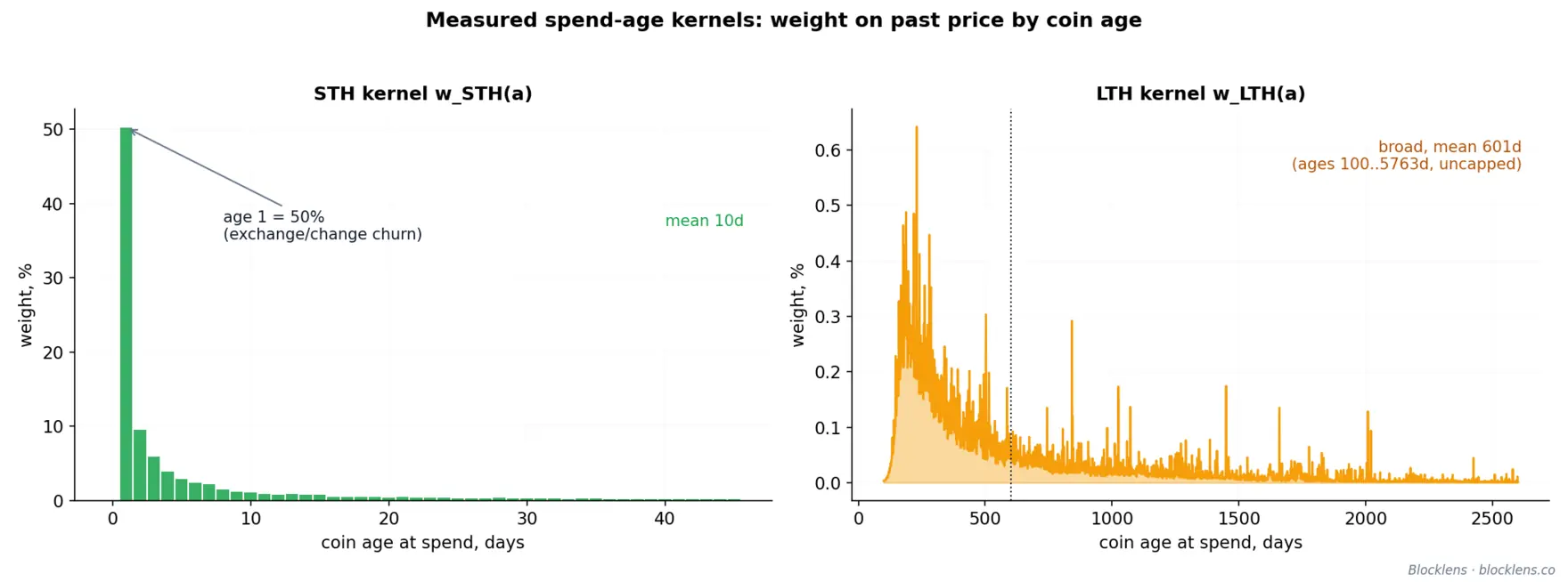
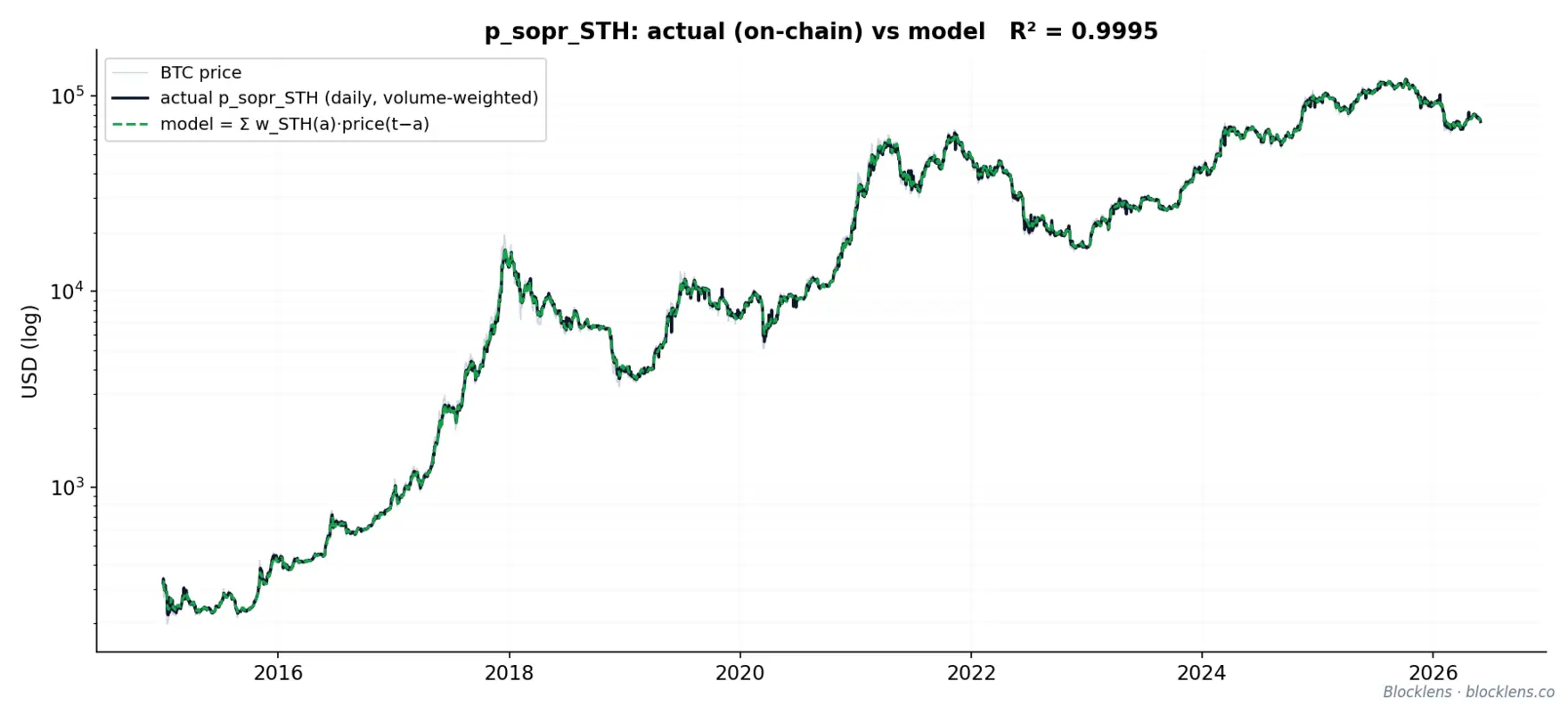
Short-term holders: a ~10-day cost basis, fit to three nines
STH spend their freshest coins, so \( p_{\text{SOPR}}^{\text{STH}} \) is a sharply front-loaded average of recent price. The front-loading is severe for a concrete reason: about \( 50\% \) of spent STH volume is one day old — coins shuffled between wallets or returned as change, moved at essentially the price they were born at, hence profit-neutral. Built from the measured kernel, the model reproduces the raw daily on-chain \( p_{\text{SOPR}}^{\text{STH}} \) almost perfectly: \( R^2 = 0.9995 \).
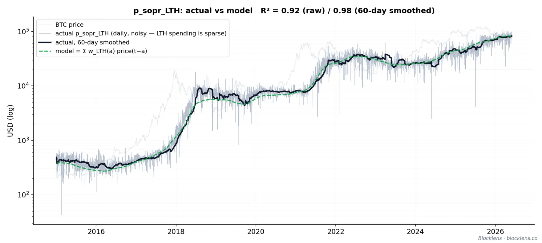
Long-term holders: a broad range, with no upper age cap
The LTH kernel is the broad spend-age distribution above, mean \( \approx 600 \) days. We deliberately impose no upper age cap: the kernel is recomputed each time from age of 100 days up to the oldest coins actually present in the data (currently out to \( \approx 5{,}760 \) days, about 15.8 years), so the cheapest, longest-dormant coins are not silently discarded when they finally move. The cost basis is
$$ p_{\text{SOPR}}^{\text{LTH}}(t) = \sum_{a} w_{\text{LTH}}(a)\, \text{price}(t - a), \tag{14}$$a broad average of price one to two years back. Long-term holders spend rarely and in bursts, so the raw daily series is genuinely noisy — the model matches it at \( R^2 = 0.92 \). Smooth the actual realized cost basis over a 60-day window and the fit rises to \( R^2 = 0.98 \). That jump in fit quality is evidence of the sparsity and irregularity of LTH spending, not a defect of the functional form.
Two cost bases, not one: the distinction between \( p_{\text{SOPR}}\) and \(\text{Realized Price}\)
Conflating SOPR and MVRV is the most common error in cohort-flow accounting. The cost basis that drives realized profit is the spent-coin cost basis \( p_{\text{SOPR}}^{g} \): the birth price of the coins that actually moved that day — an object averaging ~10 days in age for STH and ~600 days for LTH. It is what enters \( \Delta RCap\). Realized Price is the transaction-time price weighted over unspent outputs, averaging the entry price of all coins in circulation across the entire preceding history. In particular, the LTH realized price \( RP_{\text{LTH}} \), used later for the cycle bottom and the MVRV calculation, rests on an entirely different kernel — the membership-gain bell \( m(a) = W_{\text{LTH}}(a) - W_{\text{LTH}}(a-1) \), centered near 155 days, which describes when coins mature into the LTH set, not when LTH coins are spent (mean ~600 days). The cost basis \( p_{\text{SOPR}}\) asks "what did today's sellers pay for the coins they spent?"; Realized Price asks "what did everyone holding pay?" Different kernels, different questions, different places in the model.
2.2. What Moves Q: cLTH, cSTH, SLTH, SSTH
The inverse-price engine of Section 2.1 turns on a single denominator. Recall that price is reconstructed as \( p_t = \text{inertia}(t) + \Delta\mathrm{RCap}(t)/Q(t) \), where \( \Delta\mathrm{RCap}(t) \) is the daily change in Realized Cap (the realized profit or loss plus issuance) and \( Q(t) \) is the daily spend volume — the volume of coins, in BTC, that actually move and reprice that day. Everything downstream depends on how \( Q \) behaves, so it is worth knowing precisely which of its parts set its level and which set its turning points. They are not the same parts.
The spend volume decomposes into four behavioral quantities plus a protocol constant:
$$ Q(t) = c_{\text{STH}}(t)\,S_{\text{STH}}(t) + c_{\text{LTH}}(t)\,S_{\text{LTH}}(t) + \text{iss}(t), \tag{15}$$where, for each cohort \( g \in \{\text{STH}, \text{LTH}\} \), \( S_g \) is that cohort's supply (BTC held), \( c_g = V_g/S_g \) is its daily spend rate (the fraction of its holdings it moves, with \( V_g \) the BTC it spends), and \( \text{iss} \) is daily issuance in BTC.
The sensitivity law: impact = CV × weight
A driver moves \( Q \) only if it is both variable and heavy. A quantity that swings wildly but carries almost no weight in the sum cannot move the total; one that dominates the sum but never changes cannot move it either. The product of the two is what counts — and it can be written down exactly. Take any single driver and call it \( x \) — each of \( c_{\text{STH}}, S_{\text{STH}}, c_{\text{LTH}}, S_{\text{LTH}} \) in turn, one at a time. A typical daily move in \( x \) is one standard deviation, which we write as \( \delta x = \mathrm{CV}(x)\cdot x \), since the coefficient of variation \( \mathrm{CV}(x)=\sigma_x/\mu_x \) is just that deviation expressed as a fraction of \( x \) itself. To first order such a move shifts the spend volume by \( \Delta Q = (\partial Q/\partial x)\,\delta x \); divide by \( Q \) and the two effects separate cleanly:
$$ \frac{\Delta Q}{Q}\bigg|_{1\sigma} \;\approx\; \mathrm{CV}(x)\;\times\;\underbrace{\frac{\partial Q}{\partial x}\cdot\frac{x}{Q}}_{\displaystyle w_x}. \tag{16}$$The formula is evaluated separately for each driver \( x \), one row per driver. The first factor, \( \mathrm{CV}(x) \), is how much \( x \) wanders; the second, \( w_x \), is how much \( x \) matters to \( Q \) — its elasticity — and for our additive \( Q = c_{\text{STH}}S_{\text{STH}} + c_{\text{LTH}}S_{\text{LTH}} + \mathrm{iss} \) it reduces simply to the share of \( x \)'s term in the sum: \( w_{c_{\text{STH}}} = w_{S_{\text{STH}}} = c_{\text{STH}}S_{\text{STH}}/Q \approx 93\% \), and \( w_{c_{\text{LTH}}} = w_{S_{\text{LTH}}} = c_{\text{LTH}}S_{\text{LTH}}/Q \approx 7\% \). At the operating point STH turn over roughly \( c_{\text{STH}} \approx 4.2\% \) of their stack per day, LTH only \( c_{\text{LTH}} \approx 0.08\text{–}0.13\% \) — some 33 to 50 times slower — so LTH spending is only ~7% of \( Q \). Apply the law and the four contributions fall into place:
| Component | CV (range) | Weight in \( Q \) | Per-σ impact on \( Q \) | Character |
|---|---|---|---|---|
| \( c_{\text{STH}} \) | ≈ 41% (~6×) | heavy (~93%) | +38% | slow, structural |
| \( S_{\text{STH}} \) | ≈ 20% | heavy | +18% | slow, structural |
| \( c_{\text{LTH}} \) | ≈ 144% (~50×) | light (~7%) | +10% | explosive, episodic |
| \( S_{\text{LTH}} \) | ≈ 19% | light | +1% | slow, structural |
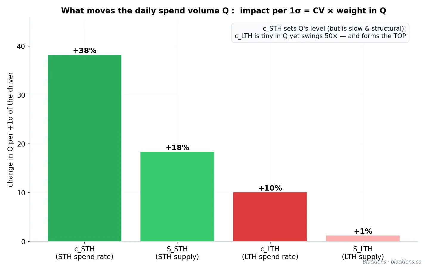
The level versus the top: why cSTH rules one and cLTH the other
The table poses a puzzle. By magnitude \( c_{\text{STH}} \) is the strongest lever on \( Q \): \( +38\% \) per σ against \( +10\% \) for \( c_{\text{LTH}} \). Jumping ahead, the model lets \( c_{\text{STH}} \) respond only weakly — a shallow, barely identifiable valuation slope — and devotes all its care to \( c_{\text{LTH}} \). The resolution is that "what sets the level of \( Q \)" and "what makes \( Q \) swell at the top" are different questions, and the cycle is decided not by Q's level but by the drivers that make it swell. The answer is not asserted; it is read off the structure of the two spend rates themselves.
Each cohort's spend rate as a function of the profitability of its unrealized positions. A simple diagnostic is to take each cohort's smoothed spend rate and plot it against that cohort's own \( \mathrm{MVRV} \) — price divided by the cohort's realized price (its cost basis) — colored by cycle. The two cohorts answer the same question with opposite signatures.
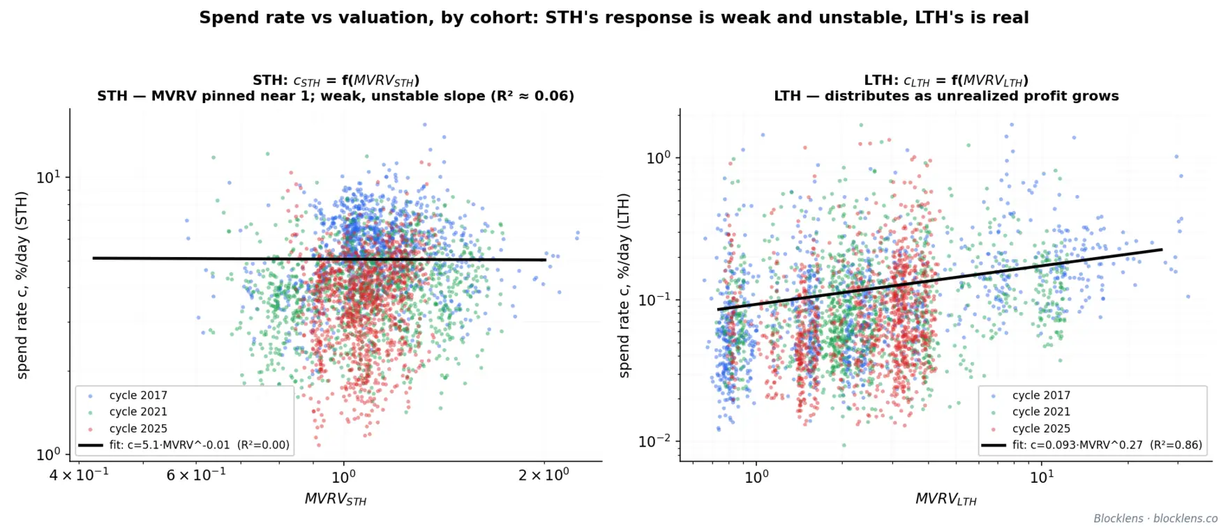
\( c_{\text{STH}} \) carries almost no cyclical information — so a near-flat law is correct. Short-term spending is market plumbing: exchange routing, change outputs, ordinary churn. It dominates \( Q \) at every moment — at the operating point \( c_{\text{STH}}\,S_{\text{STH}} \approx 156{,}000 \) BTC/day, fully 92% of a \( Q \approx 169{,}000 \) — and its level does wander (CV 41%). But across a cycle those swings capture only a small share of the profit taken out of the total capital inflow — the bulk goes to long-term holders. By construction STH sit at their cost basis, so \( \mathrm{MVRV}_{\text{STH}} \) barely leaves 1 (a ~3× range); the cohort has almost no profitability range to respond to, and what little response the fit finds carries almost no explanatory power (\( R^2 \approx 0.06\text{–}0.08 \)). \( c_{\text{STH}} \) sets where \( Q \) sits and drifts there with the microstructure of the market; it does not surge at the top, so it cannot make the top.
\( c_{\text{LTH}} \) is the driving force of the cycle. Long-term spending is the complete opposite. The cohort holds coins bought far below spot, so its profitability swings substantially across a cycle, and its spend rate rises with that profitability along a clean power law: holders wait out the entire bear market near their lows and distribute harder the further price pulls away from their cost basis. The surge is small in BTC — only ~7% of \( Q \) — but it is price-responsive and it arrives exactly when price is highest, which is when it hits the denominator hardest. This is the cyclical, profit-driven signal, and of the four drivers it is the decisive one for the turning point.
One law, both cohorts — the weak short-term response is what the fit returns. The decisive point is that treating \( c_{\text{STH}} \) as nearly flat is not an assumption imposed on the model; it is the output of the identical fitting procedure applied to both cohorts. Fit the same functional form \( c_g = A_g\cdot\mathrm{MVRV}_g^{\,b_g} \) to each cohort, parameters estimated on prior data only. The long-term exponent comes out at \( b_{\text{LTH}} \approx +0.3 \) — a real slope with genuine explanatory power (\( R^2 \approx 0.04\text{–}0.06 \) raw, \( 0.857 \) binned) acting over a 60× profitability range. The short-term exponent comes out small and unstable: about \( +0.14 \) over the full history, but anywhere from \( \approx 0 \) to \( \approx 0.3 \) depending on the window, and — decisively — with almost no explanatory power (\( R^2 \approx 0.06 \)). The same machine that finds a real, well-determined slope for LTH finds only noise for STH. A nearly flat \( c_{\text{STH}} \) is therefore not hand-tuned; it is what the data return when asked the same question — and because \( \mathrm{MVRV}_{\text{STH}} \) never leaves ≈ 1, even that shallow slope shifts \( c_{\text{STH}} \) by almost nothing across a cycle, while \( c_{\text{LTH}} \) swings by multiples.
Profit leverage: why the small cohort owns the top. LTH are only ≈ 6% of spend volume, yet they supply a rising majority of realized profit across the ascents — 36% in 2017, 54% in 2021, 68% in 2025 — because they sell coins acquired multiples below spot. At the tops the per-coin profit multiple is about \( 1.05\times \) for STH against \( 2.3\text{–}18\times \) for LTH. The cycle top is, in essence, a long-term-holder profit-taking event: a thin stream of coins carrying nearly all of the realized gain. The general lesson foreshadowed by the table holds: the variable with the most leverage on \( Q \)'s average is not the variable that forms the cycle; modeling effort follows the mechanism, not the magnitude.
Supply accounting closes the system
Before modeling \( c_{\text{LTH}} \) we reduce the unknowns: the two supplies are not independent of the spend rates — they are bookkeeping consequences of them. Total supply grows only by issuance, which is protocol-given to the satoshi:
$$ S(t) = S(t-1) + \text{iss}(t), \qquad S_{\text{STH}}(t) = S(t) - S_{\text{LTH}}(t). \tag{17}$$The cohort balances then evolve according to three conservation laws. Coins age across the "soft" 155-day boundary, producing the aging inflow \( M(t) \) (STH → LTH); long-term holders spend \( V_{\text{LTH}}(t) = c_{\text{LTH}}\,S_{\text{LTH}} \); and issuance enters as age-0 STH:
$$ S_{\text{LTH}}(t) = S_{\text{LTH}}(t-1) + M(t) - V_{\text{LTH}}(t), \tag{18}$$ $$ S_{\text{STH}}(t) = S_{\text{STH}}(t-1) + \text{iss}(t) + V_{\text{LTH}}(t) - M(t). \tag{19}$$The two cohort updates sum to \( S(t) = S(t-1) + \text{iss}(t) \) exactly, so the accounting is closed. A subtlety carries real weight: when STH spend their coins, those coins do not leave the STH pool — a spent STH coin reappears the next day as an age-0 STH coin, and a spent LTH coin recycles into the age-0 STH pool as well. So \( c_{\text{STH}} \) does not deplete \( S_{\text{STH}} \) directly (the regression coefficient of \( S_{\text{STH}} \) on \( c_{\text{STH}} \) is ≈ 0, indistinguishable from zero); it acts only indirectly, by governing how many young coins survive unspent to mature into \( M(t) \). Given the aging inflow, the entire supply block is determined by the two spend rates — and only \( c_{\text{LTH}} \) needs care.
Aging inflow. \( M(t) \) is the held portion of the short-term pool that is about to cross the soft boundary. We take the actual age structure of supply straight from the UTXO snapshots. Let \( S_{\text{age}}(t,a) \) be the amount of coins of age \( a \) days at time \( t \); then the aging inflow is that amount, weighted by the gain in LTH membership at each age:
$$ M(t) = \sum_{a=100}^{210} S_{\text{age}}(t,a)\,m(a), \qquad m(a) = W_{\text{LTH}}(a) - W_{\text{LTH}}(a-1), \tag{20}$$where \( m(a) \) is the derivative of the 155-day logistic membership function (the fraction of age-\( a \) coins crossing the boundary that day), and \( S_{\text{age}}(t,a) \) is read from the snapshots without a single fitted parameter. Most spending is short-lived churn that never matures; what crosses the boundary is not the flow volume but the quietly held stock — and it is the aging itself, not the speed of spending, that sets \( M(t) \).
Computing issuance. Daily issuance is \( \text{iss}(d) = (\text{blocks/day}) \times (\text{block subsidy}) \). The subsidy halves (the halving) on the protocol schedule (50 → 25 → 12.5 → 6.25 → 3.125 BTC) every 210,000 blocks. Blocks per day is measured per halving era as 210,000 blocks ÷ era duration: ≈ 147.4 (2009–12), 159.2 (2012–16), 149.8 (2016–20), 145.8 (2020–24). In the out-of-sample walk-forward, a cycle uses the prior completed era's block rate and projects future halving dates from it; the forward forecast runs at 145.8 blocks/day, with the next halving expected on 2028-03-30 (subsidy 3.125 → 1.5625), which lands inside the forecast window during the ascent and is included. Issuance plays three roles at once — a term in \( \Delta\mathrm{RCap} \) (\( \text{iss}\cdot p \), newly minted coins valued at spot), a term in the spend volume \( Q \), and the age-0 inflow into \( S_{\text{STH}} \).
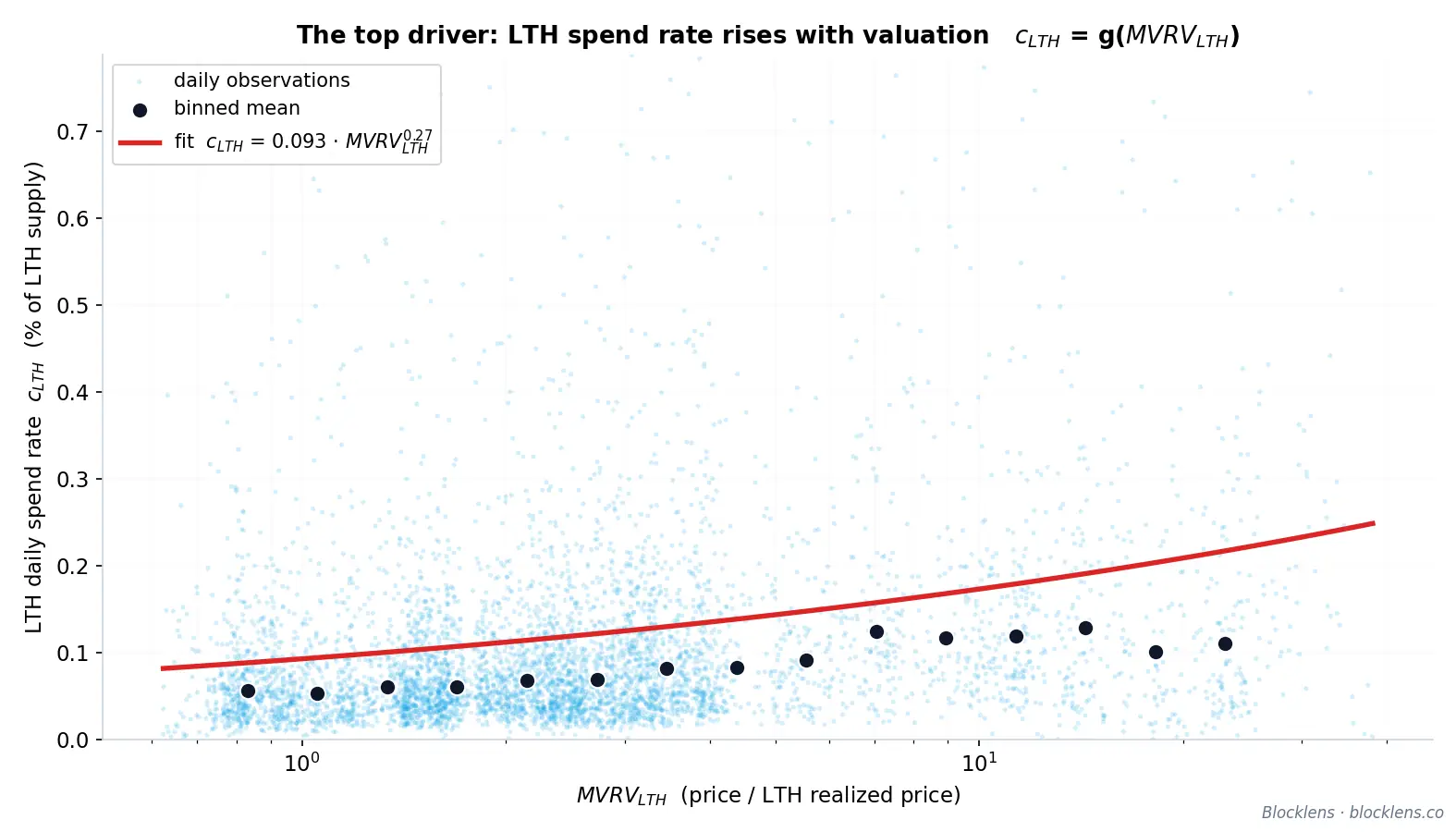
The behavioral law: cLTH = g(MVRVLTH) and the feedback that forms the top
Long-term holders distribute as a function of their unrealized profit. The natural gauge of that profit is \( \mathrm{MVRV}_{\text{LTH}} \), the ratio of the current price to the LTH realized price (the LTH cost basis): \( \mathrm{MVRV}_{\text{LTH}} = 2 \) means the cohort sits on an aggregate profit of 100% of its invested capital. The relationship is the gentle power law the scatter already showed:
$$ c_{\text{LTH}}(t) = g\!\left(\mathrm{MVRV}_{\text{LTH}}(t)\right) = 0.093 \cdot \mathrm{MVRV}_{\text{LTH}}^{\,0.27}(t). \tag{21}$$The exponent of 0.27 makes the response soft but real: distribution rises with profit, yet markedly less than proportionally — holders sell into strength gradually rather than dumping at a threshold. Binned into intervals (16 logarithmic bins), the fit holds at \( R^2 \approx 0.857 \). The fit uses a truncation \( MVRV_{LTH} \le 40 \): it excludes 92 days of early 2011 (~1.7% of the sample) where, because of the imputed birth price of coins created before market quotes existed, MVRV reaches 545 and that artifact regime destroys the law (without the truncation, \( b \approx 0.01 \)); at any reasonable threshold in the 15–100 range the exponent is stable: \( b \approx 0.27\text{–}0.30 \).
The power-law dependence of long-term-holder spending on profit is the engine of the top. It closes a negative-feedback loop that runs through the entire inverse-price identity:
- Price rises, lifting \( \mathrm{MVRV}_{\text{LTH}} \) as it pulls away from the LTH cost basis.
- Higher \( \mathrm{MVRV}_{\text{LTH}} \) raises \( c_{\text{LTH}} \) — long-term holders spend coins faster.
- The increased LTH spending enlarges the total spend volume \( Q \).
- A larger \( Q \) damps the growth of \( \Delta\mathrm{RCap}(t)/Q(t) \), so price decelerates — and rolls over into a top.
The top, in other words, is not imposed from outside by a magic multiple or a fixed price ceiling (importantly, only the date of the top is set by the cycle schedule). It is endogenous: it emerges from holders' own response to their own profit, transmitted through the supply accounting into \( Q \) and back into price. And the input with the largest variability of all, \( c_{\text{LTH}} \), earns its place not by moving \( Q \)'s level — at a 7% weight it barely can — but by moving \( Q \) in the window that decides the cycle's outcome.
Every parameter assembled in this study — the two power laws, the aging kernel, the spend-age kernels, the deployment profile of Section 2.3, and issuance — is fit on prior data only. Run that way, with no leakage, the out-of-sample walk-forward reproduces the three tops with errors of −26% (2017), +10% (2021), and −1% (2025). The model is not an oracle; these are out-of-sample errors with understood causes, and that, as Section 4 argues, is the point.
2.3. Capital-Deployment Profile and Backtests
The inverse-price engine of Section 2 turns any capital-inflow path into a price path. But to get a forecast out of it, we need to know not just how much capital a cycle deploys but when that capital arrives. That timing — the shape of the deployment curve across the ascent — turns out to be remarkably regular, and it is the last structural ingredient still missing before the full model can be backtested end to end.
The deployment profile: capital arrives back-loaded
Define the ascent fraction \( \tau \in [0,1] \) as the share of calendar time elapsed between a cycle bottom and the following top: \( \tau = 0 \) at the bottom, \( \tau = 1 \) at the top. Let \( \mathrm{frac}(\tau) \) be the cumulative deployed change in Realized Cap up to \( \tau \), expressed as a fraction of the cycle's total \( \Delta\mathrm{RCap} \). Across every modern ascent this cumulative curve collapses onto a single power law:
$$ \mathrm{frac}(\tau) = \tau^{K}. \tag{22}$$The exponent \( K \) controls how strongly capital is concentrated near the top. For \( K > 1 \) the curve is convex — deployment is back-loaded, with the bulk of fresh capital arriving in the final stretch of the run. The data are emphatic on this point: by the midpoint of an ascent (\( \tau = 0.5 \)), past cycles had actually deployed only about 7–24% of their total capital. The face-ripping part of every bull market is, quantitatively, the last act.
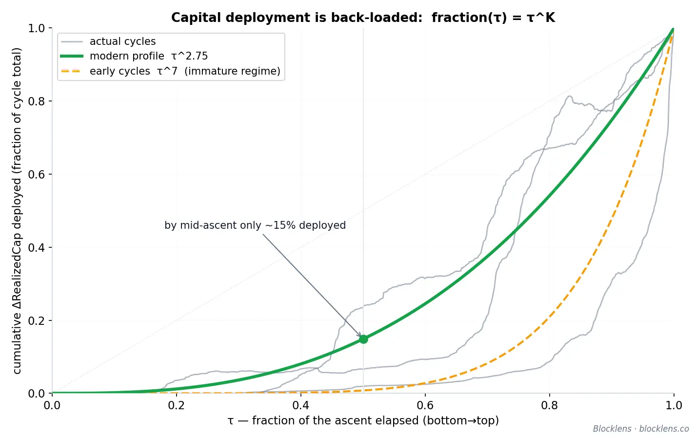
A maturation regime shift in \( K \)
The exponent is not constant across Bitcoin's history. It has fallen in a single structural step:
| Cycle regime | Representative cycles | Deployment exponent \( K \) | Interpretation |
|---|---|---|---|
| Early | 2013, 2017 | \( \approx 6.5\text{–}7.0 \) | Capital overwhelmingly concentrated in the final blow-off |
| Modern | 2021, 2025 | \( \approx 2.7\text{–}2.8 \) | Markedly more even deployment across the ascent |
The direction of the shift is intuitive. As the market deepened — more participants, more liquidity, deeper derivatives markets, and eventually spot-ETF access — capital stopped waiting for the very end of the run and began deploying more steadily across it. A lower \( K \) means a flatter, earlier inflow curve. This single number, drifting from roughly 7 toward roughly 2.75, encodes a large part of how Bitcoin's cycles have matured; we will see in Section 4 that it is precisely this parameter that makes one historical top genuinely hard to forecast.
What remains before the recursion can close
The deployment profile is the last exogenous input the engine needs — yet the loop is still not self-contained. The long-term-holder spend rate runs on \( c_{\mathrm{LTH}} = g(\mathrm{MVRV}_{\mathrm{LTH}}) \), and \( \mathrm{MVRV}_{\mathrm{LTH}} = p_t / RP_{\mathrm{LTH}}(t) \) is measured against the LTH cost basis \( RP_{\mathrm{LTH}} \) — itself a modeled quantity we have not yet built. Looking ahead, note that the very same \( RP_{\mathrm{LTH}} \) also fixes the cycle bottom.
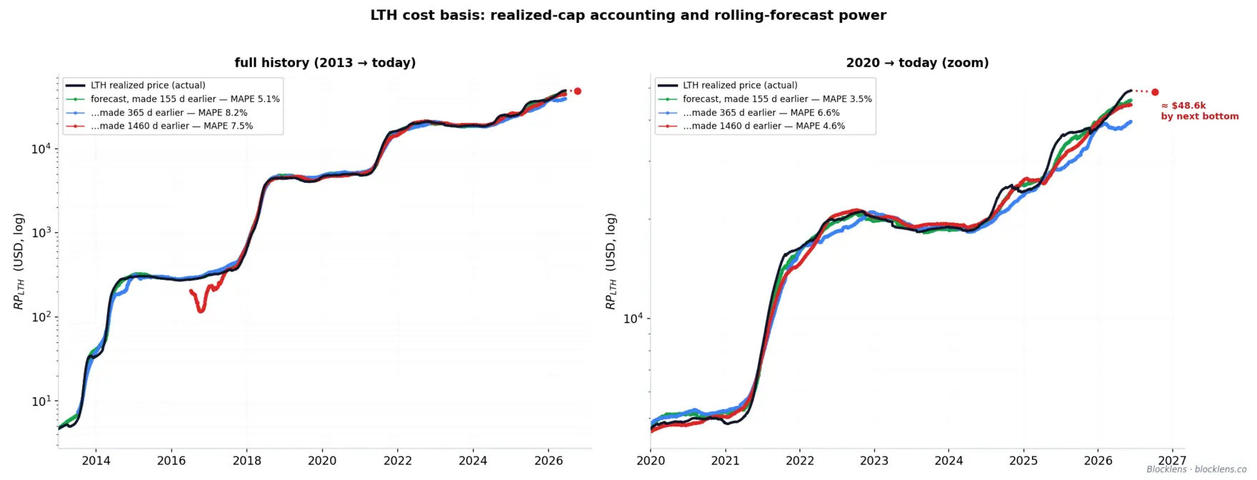
2.4. Forecasting the LTH Cost Basis (RPLTH)
Two different parts of the model lean on a single quantity: the long-term-holder cost basis, written RPLTH (the LTH realized price — the average acquisition price of all coins currently held by long-term holders). The cycle top runs on it through the distribution feedback \( c_{\mathrm{LTH}} = g(\mathrm{MVRV}_{\mathrm{LTH}}) \), where \( \mathrm{MVRV}_{\mathrm{LTH}} = p_t/RP_{\mathrm{LTH}} \); the cycle bottom is this same cost basis scaled by a floor multiple (see Section 3 for details). So before the model can close into a recursion — and before we can put a price on the next bottom — we need a forecast of where RPLTH is heading. That forecast is the subject of this section.
The good news is that RPLTH is one of the most forecastable parameters in the entire system. It moves slowly, it moves smoothly, and — crucially — it moves toward prices that have already happened. A coin that becomes a long-term holding today was bought on average about 155 days ago, the age at which its weight tips from the short-term to the long-term cohort. Its purchase price is therefore not a forecast at all; it is recorded history. The cost basis is carried forward by direct realized-cap accounting from prices that have already occurred, and the past is known.
LTH realized-cap accounting
We build the LTH cost basis not with a smoothing filter but through direct realized-cap accounting. The realized price is exactly the cohort's realized cap divided by its supply, \( RP_{\mathrm{LTH}}(t) = RC_{\mathrm{LTH}}(t)/S_{\mathrm{LTH}}(t) \), so it suffices to keep the books on \( RC_{\mathrm{LTH}} \) itself — the long-term cohort's accumulated cost basis in dollars. Each day this quantity is credited with the cost of the coins maturing into the cohort and debited by the cost basis of the coins that long-term holders spend that day:
$$ RC_{\mathrm{LTH}}(t) = RC_{\mathrm{LTH}}(t-1) + M(t)\,P_{\text{in}}(t) - V_{\mathrm{LTH}}(t)\,p_{\mathrm{SOPR}}^{LTH}(t), \qquad RP_{\mathrm{LTH}}(t) = \frac{RC_{\mathrm{LTH}}(t)}{S_{\mathrm{LTH}}(t)}. \tag{23}$$This is an ordinary accounting identity. \( M(t) \) is the daily maturation of supply into the LTH cohort (from the supply accounting of Section 2.2), and \( P_{\text{in}}(t) \) is the volume-weighted birth price of those maturing coins; their product is the realized value entering the cohort. The debit \( V_{\mathrm{LTH}}(t) \) is long-term-holder spending over the day, and \( p_{\mathrm{SOPR}}^{LTH}(t) \) is the past price of the coins spent, weighted by the spend-age kernel (that is, the cost basis leaving the cohort with them). Realized cap changes only when coins enter or exit the cohort, and each time at the price at which they once came into being; there is no spot price anywhere on the right-hand side. The LTH cost basis behaves like a supertanker — vast inertia, gentle turns — and that behavior arises on its own, because \( S_{\mathrm{LTH}} \) is large while the daily inflow and outflow are small next to the accumulated stock. There are no fitted parameters whatsoever here: both flows, \( M \) and \( V_{\mathrm{LTH}} \), and both prices, \( P_{\text{in}} \) and \( p_{\mathrm{SOPR}}^{LTH} \), are read straight from the supply accounting and the price record.
The inflow price Pin: a bell over the past
What flows in each day is not the current (spot) price but the average purchase price of the coins crossing the maturity threshold that day. Those coins do not all share one birthday. The supply aging into the LTH set on any given day was bought across a spread of earlier dates, and the shape of that spread is fixed by how the cohort weighting turns on with age.
Recall the Blocklens cohort convention: a coin of age \(a\) (days since it last moved) carries an LTH weight given by the logistic sigmoid
$$ W_{\text{LTH}}(a) = \frac{1}{1 + e^{-0.1\,(a - 155)}}, \tag{24}$$clamped to 0 below 100 days and to 1 above 210 days. The amount of supply gaining LTH membership at age \(a\) on a single day is the day-over-day increment of that weight — the membership-gain kernel
$$ m(a) = W_{\text{LTH}}(a) - W_{\text{LTH}}(a-1), \tag{25}$$which is simply the discrete derivative of the logistic curve. The derivative of a sigmoid is a bell: \(m(a)\) rises, peaks near the ~155-day midpoint, and decays away, with all of its mass falling in the 100–210-day age range. It is a smooth, single-humped weighting — a bell over recent history. This same kernel also sets the daily maturation itself, \( M(t) = \sum_{a=100}^{210} S_{\text{age}}(t,a)\,m(a) \), where \( S_{\text{age}}(t,a) \) is the actual standing amount of age-\(a\) coins read straight from the UTXO snapshots: maturation is set by the fact of aging in the already survival-filtered standing stock, not by the volume of the flow that produced it.
The inflow price is the average birth price of the maturing coins, weighted by the amount actually maturing at each age \( S_{\text{age}}(t,a)\,m(a) \):
$$ P_{\text{in}}(t) = \frac{\sum_{a} S_{\text{age}}(t,a)\,m(a)\,p(t - a)}{\sum_{a} S_{\text{age}}(t,a)\,m(a)}. \tag{26}$$In words: the coins maturing into the LTH cohort today were bought as far back as 155-plus days ago, and \(P_{\text{in}}(t)\) is the maturing-stock-weighted average (by \( S_{\text{age}}(t,a)\,m(a) \)) of what they cost. Because \(m(a)\) is concentrated around the boundary, \(P_{\text{in}}(t)\) tracks the price of roughly five to seven months ago — a window that, on the day we compute it, is entirely historical. Likewise \( p_{\mathrm{SOPR}}^{LTH}(t) \) rests only on the past birth prices of the coins being spent. Both price terms on the right-hand side of the accounting are therefore already observed by this point. This is why the bookkeeping forecasts so well: it does not predict prices — it remembers them and merely waits for them to ripen into the cost basis.
Closing the model into a recursion
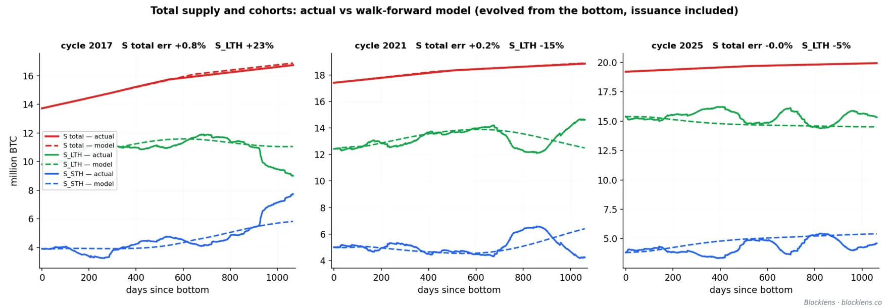
With \( RP_{\mathrm{LTH}} \) now built, the full Blocklens-TOP model closes into a self-contained recursion. From a cycle bottom we step forward day by day: the long-term-holder spend rate responds to position profitability through the distribution feedback \( c_{\mathrm{LTH}} = g(\mathrm{MVRV}_{\mathrm{LTH}}) = 0.093\cdot\mathrm{MVRV}_{\mathrm{LTH}}^{0.27} \); the relationship is fully computable since \( \mathrm{MVRV}_{\mathrm{LTH}} = p_t/RP_{\mathrm{LTH}} \) and both price and cost basis are produced by the model itself; the supply accounting of Section 2.2 updates the cohort balances and feeds the maturation \( M \) and the spending \( V_{\mathrm{LTH}} \) into the \( RC_{\mathrm{LTH}} \) accounting; the capital-deployment profile \( \tau^{K} \) of Section 2.3 supplies the day's \( \Delta\mathrm{RCap} \); and the model's final identity determines the model price. The forward STH cost basis is here derived from known parameters: \( RP_{\mathrm{STH}} = (RC_{\text{total}} - RC_{\mathrm{LTH}})/(S - S_{\mathrm{LTH}}) \), where \( RC_{\text{total}} \) is accumulated from the same \( \Delta\mathrm{RCap} \) driver. Each day's price emerges from the prior day's holder balances, cost basis, and deployed capital, run with one parameter set across all cycles and no price-fitting term anywhere in the chain. The decisive test of such a model is how it performs strictly out of sample, where every input — including the supply path and issuance — is fit only on data preceding each predicted cycle. That validation comes in Section 4, where the out-of-sample walk-forward locates the 2025 top to within 1%.
The model is good at forecasting the price potential at a cycle's top from its bottom. As of this writing, the market has not yet reached its bottom — it is still in a persistent downtrend. The logical next step is to determine the market's potential descent to its bottom and, from that point, to build the long-term forecast for the 2029 top — that is the subject of the next section.
3. A Bottom Model from Long-Term-Holder Loss
Tops and bottoms are not mirror images. A cycle top is a flow event: capital deployment decelerates as long-term holders distribute coins into strength, and the top forms when accelerating profit-taking finally outruns inflow. A bottom is something else entirely. It is not where capital stops arriving — it is where selling runs out of sellers. The distinction matters because the two extremes are governed by different quantities, and modeling a bottom as an inverted top gets the mechanism, and the number, wrong.
The cleanest evidence sits in the behavior of the Realized Cap itself. Realized Cap — the sum of every coin valued at the price it last moved — is remarkably sticky through a bear market. It barely falls. Coins do change hands during a descent, but volumes are thin, and much of the spending is holders crystallizing losses near the prevailing price, which barely changes the aggregate cost basis. The market capitalization, by contrast, collapses: a 70–80% drawdown in price erases trillions in market value while Realized Cap drifts sideways. The implication is sharp and slightly counterintuitive: a bear market is driven by market capitalization (the mark-to-market value of holders' assets), not by changes in Realized Cap (capital flowing out of the sector). The stored capital mostly does not leave; only its current mark-to-market valuation falls.
That observation tells us where to look for the floor. If realized value is conserved through the descent, the price cannot keep falling once the last seller has nothing left to spend. The natural reservoir of such sellers is the long-term-holder cohort. We track their aggregate stored cost with the LTH realized price, \( RP_{LTH}(t) \): the volume-weighted birth price of all coins currently held by long-term holders, i.e., the LTH cost basis. The ratio of spot price to that basis is the long-term-holder market-value-to-realized-value ratio, \( \mathrm{MVRV}_{LTH}(t) = p_t / RP_{LTH}(t) \), the aggregate profit multiple on long-held coins.
The loss-exhaustion floor
During a top, \( \mathrm{MVRV}_{LTH} \) is large: long-term holders sit on multiples of their cost basis and sell into strength. During the descent it falls through 1.0, the break-even line, and keeps going — the cohort as a whole moves into unrealized loss. This is the key indicator of the bottom. Selling at a loss is psychologically and economically self-limiting: the deeper the loss, the fewer holders remain willing to realize it, and the supply pressed onto the market thins to almost nothing — if anything, the impulse runs the other way, with some long-term holders inclined to average down their positions. The bottom is the point of seller exhaustion: the price at which the long-term cohort's collective position has gone so deep into drawdown that further capitulation cannot be sustained.
Empirically this point corresponds not to some arbitrary depth of drawdown but to a fairly consistent multiple of cost basis. Across every completed Bitcoin cycle, the bottom prints at an \( \mathrm{MVRV}_{LTH} \) slightly below one: for the selling to finally exhaust itself, long-term holders as a group must be carrying a real loss:
| Cycle bottom | \( \mathrm{MVRV}_{LTH} \) at the low |
|---|---|
| 2011 | 0.70 |
| 2015 | 0.66 |
| 2018 | 0.73 |
| 2022 | 0.82 |
The values cluster in a band from roughly 0.66 to 0.82; the series is non-monotone (2015's 0.66 sits below 2011's 0.70), and the “rise from cycle to cycle” rests on the last three points — a structural trend we treat as part of the broader market-maturation story (the same maturation that compresses the multiple at the top). A rising MVRVLTH at the market bottom signals that, cycle after cycle, the market reaches loss exhaustion earlier and earlier along the price decline: less unrealized drawdown is required to stop the fall, because the holder base has become deeper, more patient, and less inclined to capitulate at any given level of loss.
This gives the Blocklens-Bottom model in one line. The bottom is characterized by a fixed multiple, denoted \( \mathrm{MVRV}^{\text{floor}}_{LTH} \), applied to the long-term-holder cost basis:
$$ p_{\text{bottom}} = \mathrm{MVRV}^{\text{floor}}_{LTH} \times RP_{LTH}(t_{\text{bottom}}). \tag{27}$$The structure earns its keep. It separates a slow, forecastable quantity — the LTH cost basis \( RP_{LTH} \), which moves along a smooth, regular path extended forward by direct realized-cap accounting (which we develop in Section 2.4) — from a single empirical constant, \( \mathrm{MVRV}^{\text{floor}}_{LTH} \), calibrated to the maturation trend. Because Realized Cap — and with it \( RP_{LTH} \) — is quite sticky through the descent, the cost basis at the future bottom is largely set by the time the top is in; the model's job is simply to carry it forward with a correct RCLTH ledger and multiply by the floor.
The 365-day descent and the projected bottom
The remaining unknown in the bottom model is time — we need to know when to expect the bottom. Here Bitcoin is unexpectedly obliging: the descent from top to bottom has a remarkably stable duration. The two completed modern descents (beginning in late 2017 and late 2021) ran 363 and 366 days — within a long weekend of each other, and of a calendar year; the early-era 2013→2015 descent took 406 days and does not enter the rule, so the rule rests on two modern observations. We therefore model the descent length as approximately fixed:
$$ t_{\text{bottom}} \approx t_{\text{top}} + 365\ \text{days}. \tag{28}$$This is a regularity that has held tightly across the entire modern era (8+ years), and it gives the model a concrete date to aim at rather than an open-ended wait. We therefore place the next bottom roughly 365 days after the cycle top of October 6, 2025, i.e., around early October 2026.
Putting it together: locating the bottom
By the projected bottom date, \(RP_{LTH}\) is expected to be approximately $48,600. Taking a floor of 0.85 — a discretionary extrapolation of the rising part of the series, sitting above every value yet observed (the last: 0.82 in 2022), with an allowance for continued maturation:
$$p_{\text{bottom}} \;\approx\; 0.85 \times \$48{,}600 \;\approx\; \$41{,}300.\tag{29}$$Our central estimate for the next cycle bottom is therefore ≈ $41,300, with a floor-band range of $39,000–44,000 (allowing for the \(RP_{LTH}\) annual forecast error, MAPE 6.6–8.2%, roughly $36,000–47,000) and the low arriving in October 2026. For context, as of this report's date the market has fallen to roughly $61,700 (data cutoff June 10, 2026) — already most of the way toward the projected floor, but still holding above it.
It is worth stating plainly what makes our bottom-location method robust. We do not forecast the bottom price directly; we forecast two slow, well-behaved quantities — a valuation multiple that drifts predictably with market maturity, and a cost basis that is carried forward monotonically by direct realized-cap accounting and resists downside shocks — and let their product deliver the price. The volatile, hard-to-predict object (the dollar price at the market low) is decomposed into two stable, interpretable ones. That decomposition is the reason a bottom call can be made a year out from the top at all; and it is the same structural logic that, applied in reverse to the accelerating coin spending of long-term holders, locates the top as well.
4. Out-of-Sample Validation and the Cycle Forecast
The model was fully assembled in Sections 2–3; what remains is to test its predictive power on known historical data — with no peeking into the future — and to deliver the final forecast.
The out-of-sample walk-forward
Anyone can fit a curve to history already in hand; the real test is to name a top the model has never seen. So for each predicted cycle we re-fit every behavioral parameter on data strictly prior to that cycle, using the algorithm described in the previous sections, with no leakage from the future beyond the scalar capital-deployment figure for the full ascent (which the model does not predict but receives as a scenario input — the inflow itself is partially endogenous to price; the capital-inflow profile was taken from the prior cycle on each run). The model is conditional at its core: feed it the expected capital inflow for the cycle and it returns the implied price; it does not invent the inflow; it prices a given one.
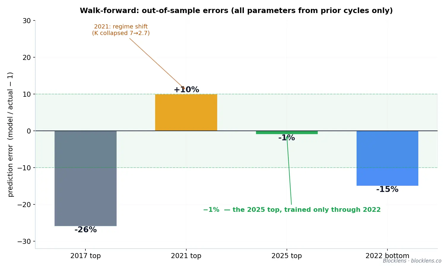
| Predicted cycle top | Out-of-sample error | Context |
|---|---|---|
| 2017 | \( -26\% \) | Early cycle; only the anomalous 2013 precedes it; capital deployment heavily back-loaded (\( K \approx 7 \)) |
| 2021 | \( +10\% \) | Regime-shift cycle: \( K \) collapsed from \( \approx 7 \) to \( \approx 2.7 \) mid-ascent |
| 2025 | \( -1\% \) | Located using only data through 2022 — the decisive test |
The 2025 result of \( -1\% \) is the headline: using nothing beyond data available by 2022, the model placed the October-2025 top within 1% of its actual value. That is predictive evidence, not a fit after the fact. The \( +10\% \) miss on 2021 is equally instructive, and we do not hide it: that cycle sat exactly on a structural break in the deployment profile — \( K \) collapsed from \( \approx 7 \) to \( \approx 2.7 \) mid-ascent — a regime shift invisible from the past. Once the new regime was established, the very next call (2025) landed within 1%.
The bottom is honestly weaker. Out-of-sample bottom errors (same accounting engine; every input prior-only — spend laws, survival curve, age kernels; the floor taken as the mean of previously observed floors): 2015 \( +30\% \), 2018 \( +25\% \), 2022 \( -15\% \). The decomposition is instructive. In 2022 the ledger nailed \(RP_{LTH}\) to within \( -1\% \) — the entire miss sits in the too-low prior-only floor forecast (0.70 against the realized 0.82). In the early cycles the picture inverts: the floor is nearly right while \(RP_{LTH}\) misses (\( +23\% \) and \( +35\% \)) — deep capitulation rewrites the cohort's cost basis faster than the ledger carries it. The bottom model's case is not an accumulated hit record but the stability of its components in the modern era: the inertia of \(RP_{LTH}\) and the maturing floor.
Timing: peak-to-peak distance
To turn a price model into a dated forecast we need a calendar — and Bitcoin is surprisingly regular here. The distance from one all-time high to the next (ATH-to-ATH, peak → peak) holds at about 1425 days, and the descent from peak to bottom is tighter still: 363 and 366 days across the two completed modern cycles (three days of spread over a span longer than a year).
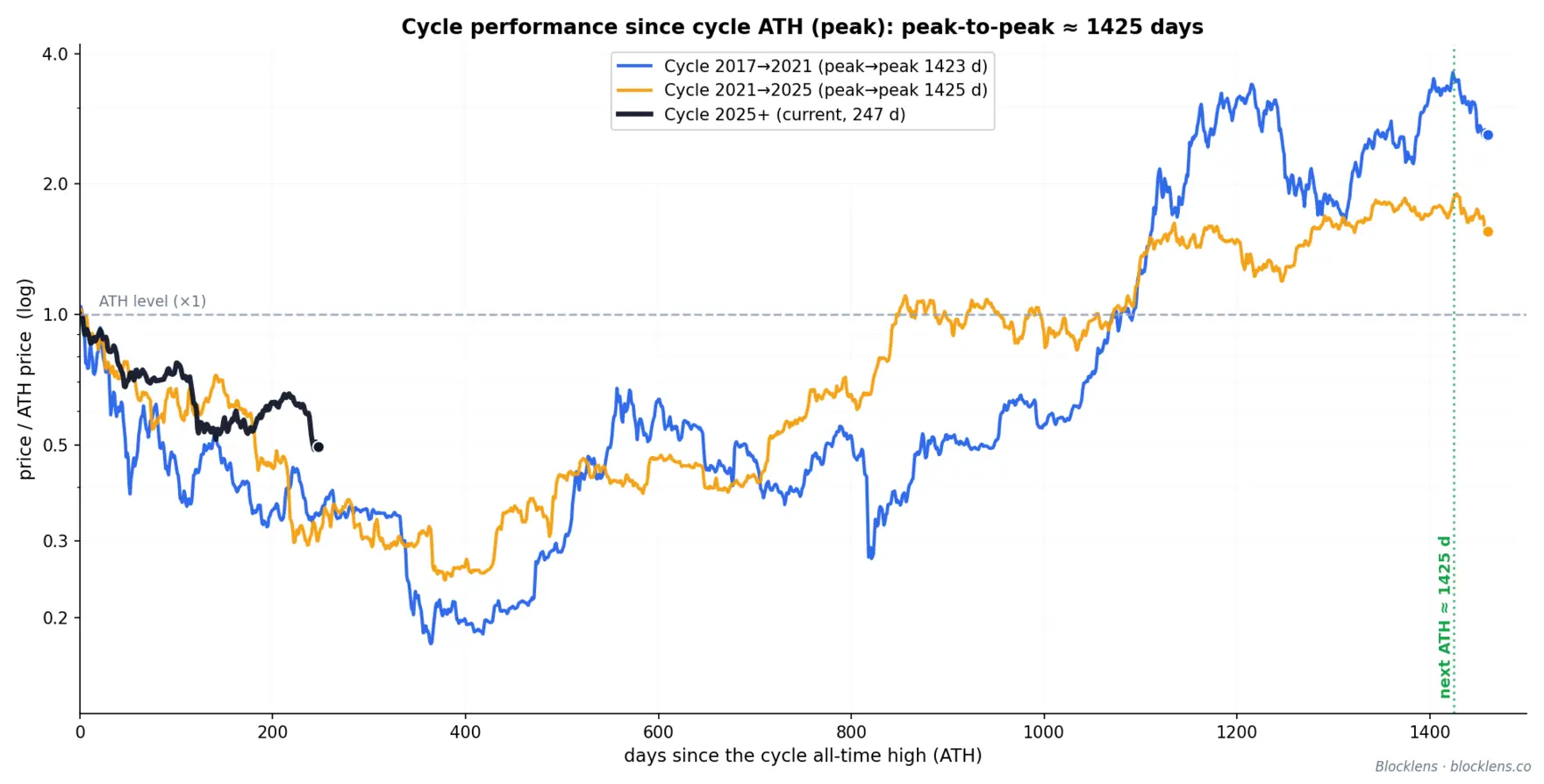
| Interval | Observed | Model convention |
|---|---|---|
| ATH-to-ATH (peak → peak) | \( \approx 1425 \) d | Full cycle length |
| Descent (peak → bottom) | 363 d, 366 d | Fixed \( \approx 365 \) d |
| Ascent (bottom → peak) | remainder | \( \approx 1060 \) d |
Applying this clock to the latest top — $124,414 on October 6, 2025 — places the cycle bottom about a year later, in early October 2026, and the next top roughly 1425 days after the previous one, in late summer 2029. The dates are fixed; the price levels remain to be filled in.
The forecast: bottom, top, and inflow scenarios
The bottom is derived in Section 3: it forms at the long-term-holder cost-basis floor, \( p_{\text{bottom}} = \text{MVRV}_{\text{LTH}}^{\text{floor}} \times RP_{\text{LTH}} \). By the forecast date the \( RC_{\text{LTH}} \) ledger carries \( RP_{\text{LTH}} \approx \$48.6\text{k} \), and a floor of \( \approx 0.85 \) gives a central bottom estimate of \( \approx \$41{,}300 \) (floor band \( \$39\text{–}44\text{k} \); with the \(RP\) forecast error — \( \approx\$36\text{–}47\text{k} \)), around October 2026.
The next top (\( \approx 2029 \)) depends on the one external input the model cannot supply itself — the cumulative capital inflow \( \Delta\text{RCap} \) over the ascent. Rather than picking scenarios out of thin air, we anchor them to the actual inflows of past cycles. From bottom to top the market deployed \$2.8B (2013), \$69B (2017), \$364B (2021), \$685B (2025). The inflow's growth multiplier decays — \( \times 24.5 \to \times 5.3 \to \times 1.88 \) — while the absolute increment has already stabilized: \( +\$295\text{B} \), then \( +\$321\text{B} \). That is the signature of a maturing asset: capital growth shifting from a multiplicative to an additive (linear) regime — and that very transition is what generates the observed multiplier decay. Each scenario below is a hypothesis about how the decay continues:
| Scenario | Hypothesis | Inflow \( \Delta\text{RCap} \) | × the 2022–2025 inflow | Implied next top |
|---|---|---|---|---|
| “Fade” (conservative) | the multiplier decay repeats | \( \$460\text{B} \) | 0.67× | \( \approx\$131\text{k} \) |
| “Maturity” (central) | the inflow increment repeats (\( +\$320\text{B} \)) | \( \$1{,}010\text{B} \) | 1.47× | \( \approx\$205\text{k} \) |
| “Momentum” (optimistic) | the prior cycle's multiplier repeats | \( \$1{,}290\text{B} \) | 1.88× | \( \approx\$242\text{k} \) |
In the conservative “Fade” scenario, the capital inflow shrinks for the first time in history — and even then the model carries price to \( \approx\$131\text{k} \), only ~5% above the 2025 top: the holder base's cost basis rises enough over the cycle that the old high is no longer expensive. The central “Maturity” scenario assumes the mature market keeps adding \( \approx\$320\text{B} \) per cycle — the linear regime, also supported by the structure of inflow channels: the coming cycle is the first with spot ETFs live from day one. “Momentum” is the upper edge: the decay pauses and the prior cycle's multiplier repeats. To be explicit: this grid is a deliberately simple extrapolation of the inflow's own history; proper inflow forecasting — incorporating macro liquidity cycles and Bitcoin's competition with other capital markets — is the subject of our future research.
The relationship inverts cleanly: the psychological BTC $500k milestone would require a cumulative \( \Delta\text{RCap} \approx \$3.3\text{T} \) (4.9× the prior cycle's inflow), a $1M coin a full \( \approx \$7.4\text{T} \) (10.8×). These are not predictions but conversion factors that translate capital-inflow expectations into price. The full trajectory — the projected \( \approx \$41\text{k} \) bottom (October 2026) and the three ascent scenarios fanning out to 2029 — is shown in the main figure.

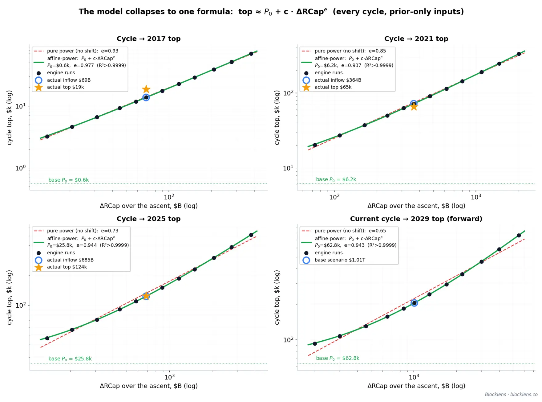
The whole model in a single formula
The model is numerical: each day's price emerges iteratively from realized-cap accounting, cohort spending, and coin maturation, and no individual part of it specifies the inflow-to-top relationship in closed form. Yet the output collapses into a remarkably simple one. Sweeping the engine across a wide grid of inflows — from 0.2× to 5.5× the actual value for each cycle, with every other input drawn from prior data only, exactly as in the walk-forward test — we find that in all four cycles the top depends on inflow through an affine-power formula with high accuracy (with a mean error MAPE of 0.2–0.4%):
$$ p_{\text{top}}(\Delta\text{RCap}) \;\approx\; P_0 \;+\; K_{100}\cdot\left(\frac{\Delta\text{RCap}}{\$100\text{B}}\right)^{e}. \tag{30}$$Here \( P_0 \) is the price at zero inflow, and \( K_{100} \) is the contribution of the first \( \$100\text{B} \) of inflow to the top price; each further \( \$100\text{B} \) adds slightly less, following a power law with exponent \( e \):
| Cycle | Base \( P_0 \) | \( K_{100} \) (first \( \$100\text{B} \) contribution) | Exponent \( e \) | \( R^2 \) |
|---|---|---|---|---|
| → 2017 top | \( \$0.6\text{k} \) | \( \$19.0\text{k} \) | 0.977 | >0.9999 |
| → 2021 top | \( \$6.2\text{k} \) | \( \$19.5\text{k} \) | 0.937 | >0.9999 |
| → 2025 top | \( \$25.8\text{k} \) | \( \$15.8\text{k} \) | 0.944 | >0.9999 |
| → 2029 top (forward) | \( \$62.8\text{k} \) | \( \$16.1\text{k} \) | 0.943 | >0.9999 |
The conversion rate of capital into price is steady: the exponent \( e \) sits in a narrow \( 0.94\text{–}0.98 \) band, and \( K_{100} \) has settled near \( \$16\text{k} \) per first \( \$100\text{B} \) in the modern era. The entire evolution of each cycle's "formula" lives in the intercept \( P_0 \) — the price at zero inflow. That is the cost-basis drift produced by internal coin turnover: old, cheap coins get spent and rewritten at current prices even without a single new dollar, so \( P_0 \) is the memory of all capital that entered before. Cycle over cycle it has grown from a negligible \( \$0.6\text{k} \) to \( \$62.8\text{k} \) — already a third of the base-case forecast. Note that a pure power law with no intercept (\( P_0 = 0 \)) fits the engine visibly worse, and its exponent drifts from cycle to cycle: the growing inherited base bends the relationship, and a fit without an intercept conflates two distinct mechanisms — inherited cost basis and fresh capital — into a single exponent.
For the upcoming cycle the formula becomes a top calculator: plug in your own estimate of cumulative inflow and read off the model-implied price without running the engine itself. Near the base scenario, every \( +\$100\text{B} \) of inflow adds \( \approx\$13\text{k} \) to the top:
$$ p_{\text{top}} \;\approx\; \$62.8\text{k} \;+\; \$16.1\text{k}\cdot\left(\frac{\Delta\text{RCap}}{\$100\text{B}}\right)^{0.943}. \tag{31}$$We stress the limits of applicability. This formula is a snapshot of the model for the 2026–2029 cycle, and it must not be blindly carried into future cycles: as the table above shows, the parameters drift systematically from cycle to cycle — above all the base \( P_0 \), which each cycle inherits from the entire prior history of capital. The 2017 formula would have said nothing about the 2025 top. It is not a replacement for the model but a convenience tool for quick calculations with it — a translation of capital-inflow expectations into the model's top price for the upcoming cycle.
5. Conclusions, Limitations & Next Steps
Forecasting a complex system can always be made simpler by tracing its interdependencies and driving factors. For Bitcoin, the fuel for price is capital inflow, and its best available estimate is the change in Realized Cap: the metric is nearly smooth, moves slowly, and carries more than 15 years of accumulated history. It is comparatively easy to form a view of how interest in the crypto-asset sector — and with it, indirectly, the capital inflow — will change relative to the previous cycle.
All too often, analysts' Bitcoin valuations are pulled out of thin air or rest on statistically insignificant technical-analysis metrics. The careful, methodologically rigorous approach behind the Blocklens-TOP model lets us screen out estimates of that kind: we consider Bitcoin reaching $1M before 2030 unrealistic, for example, and a break above $500k in the same period unlikely (assuming dollar inflation holds at its current level), because that would require, within a fairly short 3-year window (from bottom to top), capital inflows on a scale observed in only a handful of asset classes in all of human history (the U.S. Treasury market, China's new-build housing market of 2019–2021, U.S. war bonds during World War II, and so on).
What the model is
Three properties define it.
It is mechanistic, not statistical. Price is recovered from the inverse-price relation \( p_t = \text{inertia}(t) + \Delta\text{RCap}(t)/Q(t) \), where \(Q(t)\) is the daily spend volume in BTC and the inertia term is the spend-weighted cost basis of the coins moving that day. Nothing here is a black box. Each quantity — cohort supply, spend rate, cost basis — is an observable on-chain metric with economic meaning.
The top is endogenous. The model discovers the top on its own, from a single negative feedback loop. As price rises, the LTH market-value-to-realized-value ratio (MVRVLTH, price divided by the LTH cost basis) rises with it, and long-term holders distribute faster according to a gentle power law,
$$ c_{\text{LTH}}(t) = g\!\left(\text{MVRV}_{\text{LTH}}(t)\right) = 0.093 \cdot \text{MVRV}_{\text{LTH}}^{0.27}(t) \quad (\text{binned } R^2 \approx 0.857). \tag{32}$$Faster distribution lifts the daily spend volume \(Q\), which damps the growth of \(\Delta\text{RCap}/Q\), which in turn decelerates price into a top. The very behavior that marks euphoria is the behavior that ends it.
It validates out-of-sample on the modern regime. Under a strict out-of-sample walk-forward — every input refit on data strictly prior to each predicted cycle, with no future leakage, including the supply path and issuance — the model locates the 2025 top to within 1% (an error of −1%), using only data through 2022 plus the exact value of the future capital inflow. The actual 2025 top printed at $124,414. That single number is the headline result of this work: a price-formation model with every behavioral parameter fit only on data through 2022, given the actual cycle inflow total and calendar, reproduces the peak three years (one full bull market) into the future to within 1% — with every input, supply dynamics included, fit exclusively on prior data.
What the model is not
Being clear about a model's reach is part of its specification. The Blocklens-TOP model is powerful precisely because it is narrow, and it is worth being explicit about the edges.
It is not an autonomous oracle. The engine maps capital inflow to price; it does not forecast the inflow. The cumulative deployment of \(\Delta\text{RCap}\) across an ascent follows \( \text{frac}(\tau) = \tau^{K}\), where \(\tau\) is the fraction of the ascent elapsed — strongly back-loaded, with only ~7–24% of capital deployed by mid-ascent. Every forward price path is therefore conditional on a total-inflow scenario. State the scenario and the model returns the top: $460B of cycle inflow (“Fade”) implies ~$131k, $1.01T (“Maturity”) ~$205k, $1.29T (“Momentum”) ~$242k. Run it in reverse and BTC at $500k requires \(\Delta\text{RCap} \approx \$3.3\text{T}\), while $1M demands ~$7.4T. These are not predictions; they are the exchange rate between deployed capital and price, and the capital itself remains an input.
Regime shifts are intrinsically hard. The deployment exponent \(K\) is not constant across history. Early cycles deployed capital far more unevenly (\(K \approx 6.5\text{–}7.0\) in 2013 and 2017); modern cycles have a flatter profile (with successive sigmoid bursts visible along it): \(K \approx 2.7\text{–}2.8\). The 2021 cycle sits squarely on the fault line: \(K\) collapses from ~7 to ~2.7 mid-ascent — a structural break that was unknowable from prior data. The out-of-sample walk-forward shows its cost plainly: the 2021 top overshoots by +10%. The model cannot foresee a regime change; it can only price one once the new regime is legible.
The sample is small. Bitcoin has lived through roughly five cycles. No amount of statistical care manufactures degrees of freedom that the data does not contain, and every out-of-sample claim here should be read with that ceiling in mind. The encouraging signal — the part that suggests the engine captures real structure rather than coincidence — is that out-of-sample the modern tops land at +10% (2021) and −1% (2025), and the bottoms more loosely: +30% (2015), +25% (2018), −15% (2022), with the modern bottom miss explained entirely by the floor rather than the cost basis — all with every input fit solely on data preceding the predicted cycle.
Next steps
The model is a foundation, and several potential improvements follow naturally from the point where it currently stops.
- A multi-factor model for predicting the spend rate. The power law for \(c_{\text{LTH}}\) is a simplification (it depends on a single factor: the profitability of long-term holders' positions). In reality, long-term holder behavior is always shaped by several factors at once (return expectations, price momentum, time within the cycle, and so on). More sophisticated and more accurate models for \(c_{\text{LTH}}\) are the subject of our future research.
- Forecasting the capital inflow and its distribution over time. Section 4 uses a fairly primitive set of scenarios for possible capital inflows. The inflow itself — and interest in the crypto-asset sector — clearly depends on macroeconomic factors and the state of adjacent capital markets. In future versions of the Blocklens-TOP model we will try to close this gap and couple the two models, yielding a complete picture.
- Live tracking. All inputs derive from Blocklens daily UTXO age-cohort snapshots and holder-valuation metrics, so the entire model can run as a continuously updating monitor — tracking the descent now unfolding (mid-2026 price near $61.7k against the 2025 top of $124,414) into the projected bottom, and re-pricing the next ascent as capital-inflow data arrives.
The Blocklens-TOP model will not tell you the future on its own — and it does not pretend it can. What it does is convert a question no one can answer — where will the price go? — into one that is at least tractable: how much capital will be deployed? Answer that, and the rest is simple arithmetic.
6. Glossary of Terms and Symbols
Every symbol and abbreviation used in this report is collected here. The entries are grouped for ease of navigation: market and on-chain primitives first, then the cohort machinery, the inverse-price engine, the top driver, and finally the bottom and cycle constructs. Subscript \(g\) ranges over the two cohorts \(\{\text{STH},\text{LTH}\}\); \(t\) denotes a day and \(a\) a coin's age in days.
6.1 Market and on-chain primitives
| Term / symbol | Definition |
|---|---|
| BTC | Bitcoin, the native asset; also the unit in which coin quantities (supply, spend, issuance) are measured. |
| UTXO | Unspent Transaction Output — an on-chain coin parcel of a given BTC amount that carries the timestamp of its last move; the atomic unit of all cohort accounting here. |
| coin age, \(a\) | Days elapsed since a UTXO last moved; the variable by which a coin is classified as short- or long-term held. |
| price, \(p_t\) | BTC spot closing price in USD on day \(t\). |
| issuance, \(\text{iss}\) | New BTC minted by the protocol per day (the block subsidy summed over the day), valued at \(p_t\) when added to realized capital. |
| Market Cap | Circulating supply valued at the current spot price, \(S(t)\cdot p_t\); the "paper" valuation of the network. |
| Realized Cap (RCap) | Supply valued at each coin's last-moved price rather than spot — the aggregate USD cost basis of all coins; the capital actually committed on-chain. |
| \(\Delta\text{RCap}(t)\) | Daily change in Realized Cap; equals realized profit/loss on spent coins plus issuance valued at the spot price (the core identity). |
| Realized Price (RP) | Realized Cap divided by supply — the average cost basis per coin, in USD. Computed per cohort, it gives the cohort cost basis (see \(RP_{\text{LTH}}\)). |
| \(RP_{\text{LTH}}\) | LTH realized price — the long-term-holder cost basis (Realized Cap of LTH coins divided by LTH supply); the anchor of the bottom model and the quantity that realized-cap accounting forecasts. |
| MVRV | Market-Value-to-Realized-Value ratio, \(\text{Market Cap}/\text{Realized Cap}\) (equivalently \(p_t/RP\)); a dimensionless gauge of aggregate unrealized profit. |
| MVRVLTH / MVRVSTH | MVRV computed within a single cohort, \(p_t/RP_g\); MVRVLTH (price over the LTH cost basis) governs long-term-holder distribution and acts as the defining driver of both the top and the bottom. |
| SOPR | Spent Output Profit Ratio — for the coins moved on a given day, the sale price divided by the price at which those same coins were acquired; SOPR \(>1\) means the day's spenders realized a profit on average. |
| \(p_{\text{SOPR}}^{g}\) | SOPR cost basis of cohort \(g\): the volume-weighted birth price of the coins that cohort actually spent that day, \(p_{\text{SOPR}}^{g}=p_t-\Delta\text{RCap}_g/V_g\). This spent-coin cost — not the holdings cost — is what enters the realized-P/L term. |
6.2 Cohorts and the age-weighting kernels
| Term / symbol | Definition |
|---|---|
| cohort | One of the two age-defined holder classes into which every coin is split by value: Short-Term Holders and Long-Term Holders. |
| STH | Short-Term Holders — recently moved coins (low age); high turnover; they spend their freshest coins first. |
| LTH | Long-Term Holders — coins held long enough to dominate the upper age range; sparse spenders whose acceleration forms cycle tops. |
| \(W_{\text{LTH}}(a)\) | Logistic age weight assigning a coin's LTH membership fraction, \(W_{\text{LTH}}(a)=1/\!\left(1+e^{-0.1(a-155)}\right)\), clamped to 0 below 100 days and 1 above 210 days; \(\sim\!155\) days is the soft STH/LTH boundary, with \(W_{\text{STH}}(a)\) \(=1-W_{\text{LTH}}(a)\). |
| \(m(a)\), membership-gain kernel ("the bell") | Daily LTH membership gained at age \(a\), \(m(a)=W_{\text{LTH}}(a)-W_{\text{LTH}}(a-1)\) — the discrete derivative of the logistic sigmoid, a bell-shaped curve over ages \(\sim\!100\text{–}210\) days. It is the age distribution of coins entering the LTH set each day, and hence the natural kernel for the LTH cost basis. |
| \(S_g\), supply | Total BTC held by cohort \(g\); \(S(t)=S_{\text{STH}}(t)+S_{\text{LTH}}(t)\), with total supply \(S(t)\) protocol-given. |
| \(V_g\) | BTC spent (moved) by cohort \(g\) on a given day. |
| \(c_g\), spend rate | Cohort daily spend rate, expressed as a percentage, \(c_g=V_g/S_g\) — the fraction of a cohort's holdings transacted that day. Operating ranges: \(c_{\text{STH}}\approx 4.2\%/\text{day}\), \(c_{\text{LTH}}\approx 0.08\text{–}0.13\%/\text{day}\). |
| \(M(t)\), aging inflow | STH\(\rightarrow\)LTH maturation flow: BTC crossing into the LTH set per day as coins age, \(M(t)=\sum_a S_{\text{age}}(t,a)\,m(a)\) — read endogenously from the actual age structure of supply (historically \(\sim\!16.3\)k BTC/day on average); the source term that grows LTH supply. |
6.3 The inverse-price engine and the top driver
| Term / symbol | Definition |
|---|---|
| \(Q(t)\), daily spend volume | Daily spend volume in BTC, \(Q(t)=c_{\text{STH}}(t)S_{\text{STH}}(t)+c_{\text{LTH}}(t)S_{\text{LTH}}(t)+\text{iss}(t)\) — the total coin volume across which the day's capital flow is spread; the denominator of the inverse-price relation. |
| inertia | Spend-weighted cost basis of the day's movers, \(\text{inertia}=(c_{\text{STH}}S_{\text{STH}}\,p_{\text{SOPR,STH}}+c_{\text{LTH}}S_{\text{LTH}}\,p_{\text{SOPR,LTH}})/Q\); the price level toward which the engine reverts before capital flow pushes it, giving \(p_t=\text{inertia}(t)+\Delta\text{RCap}(t)/Q(t)\). |
| CV | Coefficient of variation — standard deviation over mean, the unit-free variability of a driver (e.g., the CV of \(c_{\text{LTH}}\) \(\approx 144\%\)). |
| sensitivity law | A driver's per-\(\sigma\) impact on \(Q\) equals its CV times its weight in \(Q\); thus \(c_{\text{STH}}\) sets \(Q\)'s level while \(c_{\text{LTH}}\), small in weight but huge in variability, forms the top. |
| \(g(\cdot)\), distribution feedback | The top driver: LTH spend rate as a power law of MVRVLTH, \(c_{\text{LTH}}=g(\text{MVRV}_{\text{LTH}})=0.093\cdot\text{MVRV}_{\text{LTH}}^{0.27}\) (binned \(R^2\approx 0.857\)). A negative feedback: higher price raises MVRV, speeds LTH selling, lifts \(Q\), and decelerates price into a top. |
6.4 Capital deployment, the bottom, and cycle shape
| Term / symbol | Definition |
|---|---|
| \(\tau\) | Fraction of an ascent elapsed, from 0 at the bottom to 1 at the top; the clock of the deployment profile. |
| \(K\), deployment exponent | Curvature of cumulative capital deployment, \(\text{frac}(\tau)=\tau^{K}\) (share of the cycle's total \(\Delta\text{RCap}\) deployed by \(\tau\)); larger \(K\) means more back-loaded deployment. Modern cycles \(K\approx 2.7\text{–}2.8\); early cycles \(K\approx 6.5\text{–}7.0\). |
| \(\text{MVRV}_{\text{LTH}}^\text{floor}\) | The MVRVLTH level at which long-term holders' aggregate position is deep enough underwater that selling exhausts itself — the bottom condition. Empirically \(0.70\) (2011), \(0.66\) (2015), \(0.73\) (2018), \(0.82\) (2022), rising over cycles; the report uses \(\approx 0.85\) going forward. |
| \(p_{\text{bottom}}\) | Modeled cycle low, \(p_{\text{bottom}}=\text{MVRV}_{\text{LTH}}^\text{floor}\times RP_{\text{LTH}}(t_{\text{bottom}})\), reached at \(t_{\text{bottom}}\approx\text{top}+365\) days (modern descents lasted 363 and 366 days). |
| \(P_{\text{in}}(t)\) | Average birth price of coins maturing into the LTH set on day \(t\), weighted by the maturing amount: \(P_{\text{in}}(t)=\sum_a S_{\text{age}}(t,a)\,m(a)\,p_{t-a}\big/\sum_a S_{\text{age}}(t,a)\,m(a)\); the input that the RCLTH ledger accounts for. |
| ATH | All-Time High — the highest price ever recorded up to a given date (the 2025 cycle top was \$124,414). |
| drawdown | Percentage decline from a prior peak (ATH) to a later trough; the depth of a bear market, which compresses as the market matures. |
| capitulation | The phase of forced, loss-realizing selling near a bottom, when holders surrender coins below cost and unrealized loss is exhausted. |
| MAPE | Mean Absolute Percentage Error — the average of \(|\hat{y}/y-1|\) across all forecasts, expressed in percent; a standard measure of forecast accuracy in which positive and negative misses do not cancel out. A MAPE of 5% means the forecast deviates from the actual value by 5% on average, in either direction. |